Miguel Neves
580 California St., Suite 400
San Francisco, CA, 94104
2010, Shock and Vibration
https://doi.org/10.1155/2010/630942This paper reports on the modeling and on the experimental verification of electromechanically coupled beams with varying crosssectional area for piezoelectric energy harvesting. The governing equations are formulated using the Rayleigh-Ritz method and Euler-Bernoulli assumptions. A load resistance is considered in the electrical domain for the estimate of the electric power output of each geometric configuration. The model is first verified against the analytical results for a rectangular bimorph with tip mass reported in the literature. The experimental verification of the model is also reported for a tapered bimorph cantilever with tip mass. The effects of varying cross-sectional area and tip mass on the electromechanical behavior of piezoelectric energy harvesters are also discussed. An issue related to the estimation of the optimal load resistance (that gives the maximum power output) on beam shape optimization problems is also discussed.


![TABLE 1: Geometric and material properties of the bimorph harvester. n the first case, the model is verified against the analytical results of a bimorph cantilever with tip mass reported in the iterature [13]. The experimental verification of the model is then reported for a tapered bimorph cantilever with tip mass. Finally, a discussion regarding the calculation of the optimal oad resistance (for maximum power output) is presented. The effects of varying cross-sectional area, tip mass, and estimate of optimal load resistance on the electromechanical behavior and shape optimization problems of piezoelectric energy harvesters are also discussed. It is important to mention that, in the following discussions, the power output is normalized per base acceleration (in terms of gravitational acceleration), which is assumed to be smaller than that which would cause failure in the different piezoelectric energy harvesters considered in this work.](https://figures.academia-assets.com/46494565/table_001.jpg)


![2.2. Modal Parameter Estimation. All modern, commercia algorithms for estimating modal parameters from exper- imental input-output data utilize matrix coefficient, poly- nomial models. This general matrix coefficient, polynomia’ formulation yields essentially the same polynomial form for both time and frequency domain data. Note, however, that this notation does not mean that, for an equivalent mode order, the associated matrix coefficients are numerically equal. The size of the square, matrix coefficients ([«]), and the order of the polynomial (m) vary with the algorithm. Once the matrix coefficients ([a]) have been found, the modal frequencies (A, or z,) can be found as the roots of the matrix coefficient polynomial (see (3) or (5)) using any one of a number of numerical techniques, normally involving an eigenvalue problem of the companion matrix associated with the matrix coefficient polynomial.](https://figures.academia-assets.com/46494565/figure_045.jpg)

![TABLE 2: Four corners of modal parameter estimation. order form. A recent paper explains that the two methods are theoretically equivalent [8].](https://figures.academia-assets.com/46494565/table_005.jpg)


![Figure 3: Extended consistency diagram, conventional version. challenging. Based upon the construction of the disc, real- valued, normal modes can be expected and the inability to resolve these modes can be instructive relative to both modal parameter estimation algorithm and autonomous procedure performance. For the interested reader, a number of realistic examples are shown in other past papers including FRF data from an automotive structure and a bridge structure [9, 16].](https://figures.academia-assets.com/46494565/figure_049.jpg)
![Figure 4: Extended consistency diagram, pole-weighted MAC version. Figure 4 is an example using a pole-weighted vector (state vector) method of producing a similar consistency diagram. This approach is easier to implement numerically and provides equal or better results when compared to the conventional approach for almost all cases. In this example, every estimate from every matrix coefficient polynomial solution from every algorithm is converted into a pole- weighted vector of a specific order, in this case tenth order. Then, the consistency diagram is developed by using the same vector correlation methods (MAC) [17, 18] to iden- tify consistency without a need for a separate consistency comparison for frequency and damping (since the modal frequency is included in the pole-weighted vector). A similar set of symbols, as those used in Figure 3, are used to define increased levels of vector consistency in terms of the MAC value between all pole-weighted vectors.](https://figures.academia-assets.com/46494565/figure_050.jpg)


![large systems, it is a nontrivial task. For this reason, a lot of formalisms have been developed. Numerical formalisms especially play a significant role as they are used in computer multibody codes which becomes more and more popular and sophisticated [9].](https://figures.academia-assets.com/46494565/figure_053.jpg)


![The optimal input force moves can be obtained as the solution of an unconstrained optimization problem (minimization) with the following cost function [24]: definite or at least one is positive definite and the other is semipositive definite.](https://figures.academia-assets.com/46494565/figure_079.jpg)


![where b,, is the mode shape for mode n and y, is a vector describing the modal participation of the considered mode. It is important to note that the negative time part of the correlation function matrix R,_(t) is in fact a free decay because it is written as a linear combination of modal contributions (terms proportional to the mode shape times a complex exponential), whereas the positive time part R,, (7) is in fact only a free decay if it is used in its transposed form so the terms y,b2 turn into the form bv. and the response becomes proportional to the mode shapes. This means that whenever correlation functions are used as free decays, using the positive part of the correlation function matrix, the matrix must be used in its transposed form. It should also be noted that if we had not followed the definition given by (5) but instead defined the correlation matrix as R(t) = E[y(t + ny’ (t)] which is common in some presentations of random vibration theory, then because of stationarity this is equal to Ely(t)y" (t —T)].So this swaps the time of the solutions for the correlation function matrix in (17), and thus in this case the positive part of the correlation function matrix can indeed be used as free decays without taking the transpose. Other central relations in random vibrations are the modal decompositions of the correlation function and PSD function matrices. The modal decomposition of the correla- tion function matrix is due to James et al. [6]. Expressing a general response by its modal decomposition and assuming white noise input where the correlations functions all degen- erate to the Dirac delta functions it can be shown that the correlation function matrix for negative times R,_(t) and for positive times R,,, (tT) is given by](https://figures.academia-assets.com/46494565/figure_091.jpg)
![correlation functions and the free decays are then arranged in a Hankel matrix, Vold et al. [11, 12], Here the operating responses y(n) are given in terms of the discrete time t,, = nAt. The matrix containing the AR matrices of the free decays](https://figures.academia-assets.com/46494565/figure_092.jpg)
![We can then estimate the observability and controllability matrices as follows: In ERA two Hankel matrices are formed, Juang and Pappa 16] and Pappa et al. [17, 18],](https://figures.academia-assets.com/46494565/figure_093.jpg)


![n this paper, a new MPC connection element is defined, which enables to create an interface between the concept D beam model and the detailed 3D joint model, as shown in Figure 3. For such purpose, the kinematic relationships between the displacements and rotations of the beam node (dependent node of the connection element) and the dis- placements of the nodes of the detailed 3D FE model of the joint at the interface section (independent nodes of the connection element) are derived in the form of a transformation matrix [R], by using a static approach based on equilibrium conditions [11]. The basic idea is to obtain a second transformation matrix [S] that defines the relationship between the total forces at the central node of the beam/joint interface and the nodal loads over the section, considering theoretical stress fields resulting from the Saint- Venant assumptions with respect to axial, bending, shear, and torsion load-cases for a beam-like structure [12]. In linear elastic field, this loads correlation can be inverted, returning the searched kinematic relationship. where {o} is the vector of nodal stresses, [S,] is the stress recovery matrix, and {F} is the vector of total forces applied to the central node. In particular, (1) for a generic rectangular cross-section can be detailed as follows: The physical meaning of each parameter is given in Table 1.](https://figures.academia-assets.com/46494565/figure_098.jpg)
![where {f} is the vector of total nodal forces, [S,] is the form nodal load matrix, and {o} is the vector of total nodal stresses. In extended notation, (5) can be rewritten as follows: Note that, for open sections, the forces applied on internal nodes receive the contribution of average stresses relating to both adjacent elements; instead, external nodes belong to a single element and then their values are considerably lower. Therefore, by combining (1) and (5), it is possible to obtain the relation between the total forces at the central node, {F}, and the nodal forces on the outer contour of the section {f}: To obtain the [R] matrix that relates 1D beam displace- ments and rotations and 3D displacement values at the interface, linear relations between forces and displacements are assumed. In this way, it is sufficient to transpose [S]: Since the average stresses at the interface are constant, the nodal loads for i and j can be calculated by using shape functions, yielding](https://figures.academia-assets.com/46494565/figure_099.jpg)


![Ficure 5: Profile of detailed 3D beam model: a generic shell element k and the two nodes at interface, i and j [11]. Figure 4: Stress distribution along rectangular cross-sections, due to vertical shear (t,,, and T,, in (a)) and warping torsion (a, in (b)): the global effect of linear parts in the central node is zero.](https://figures.academia-assets.com/46494565/figure_102.jpg)


![Ficure 13: Vertical displacements of the vehicle/track contact points at the speed 30 m/s [1], 12].](https://figures.academia-assets.com/46494565/figure_118.jpg)
![Figure 14: Vertical displacements of the vehicle/track contact points at the speed 50 m/s [1], 12].](https://figures.academia-assets.com/46494565/figure_119.jpg)

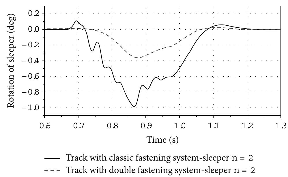
![Ficure 16: Vertical displacements of rails registered 180 cm in front of the contact points of the buggy for classic and “Y”-type track at the speed 40 m/s [12]. References Ficure 15: Vertical displacements of rails registered 120 cm in front of the contact points of the buggy for classic and “Y”-type track at the speed 40 m/s [12].](https://figures.academia-assets.com/46494565/figure_121.jpg)


![The position vector of the satellite mass center with respect to the inertial reference system (x, y, z) (see Figure 1) is Details of the equations of motion derivation can be found in [12], where L is the Lagrangian of the system, the generalized coordinates are V and a, R is the Rayleigh dissipation function, tT, is the internal torque, and 1, is the external torque. Assume that R,T,, T,,w, V are given by](https://figures.academia-assets.com/46494565/figure_128.jpg)


![TABLE 2: Frequency range (Hz) for different patterns of movement (adapted from [14]). one attends to the frequency of movement, resulting from a speed of 0.5 m/s to 0.8 m/s (for slow walk) to 3.5 m/s (for jogging-slow running) with a step size from 0.65 m for slow walk and not exceeding 1.7 m for fast running (Table 2).](https://figures.academia-assets.com/46494565/table_021.jpg)
![FiGure 7: (a) Force-time typical diagram for different movements: left-step frequency < 2.2 Hz, right-step frequency > 2.2 Hz; (b) variation in time-space imposed by the walking movement [15].](https://figures.academia-assets.com/46494565/figure_141.jpg)


![Figure 10: (a) Allowable vertical accelerations as a function of frequency of vertical mode [26], (b) frequencies to be avoided [14, 17]](https://figures.academia-assets.com/46494565/figure_144.jpg)
![TABLE 4: Acceleration limits recommended in some codes (Figure 10(a)). Zivanovié et al. [11], Heinemayer et al.[29], SETRA [30], and HIVOSS Project [2] are three important references summarizing topics and restrictions for comfort and safety of footbridges. More recent advancements were produced and are presented in publications such as Footbridge-2008 [31] and Footbridge-2011 [32]. one instrument), the agreement is very good, also for high frequency modes.](https://figures.academia-assets.com/46494565/table_023.jpg)

![T Values of vertical accelerations exceeding the less stringent limit (93.8 mg); *the most stringent limit (66.7 mg); “values exceeding the code ones for horizontal vibrations (20 mg, EN 1990 [20]).](https://figures.academia-assets.com/46494565/table_025.jpg)

![TABLE 8: Peak acceleration amplitudes for different tests. ' Values exceeding the code limits for horizontal vibration (20 mg). EN-1990 [20]).](https://figures.academia-assets.com/46494565/table_027.jpg)


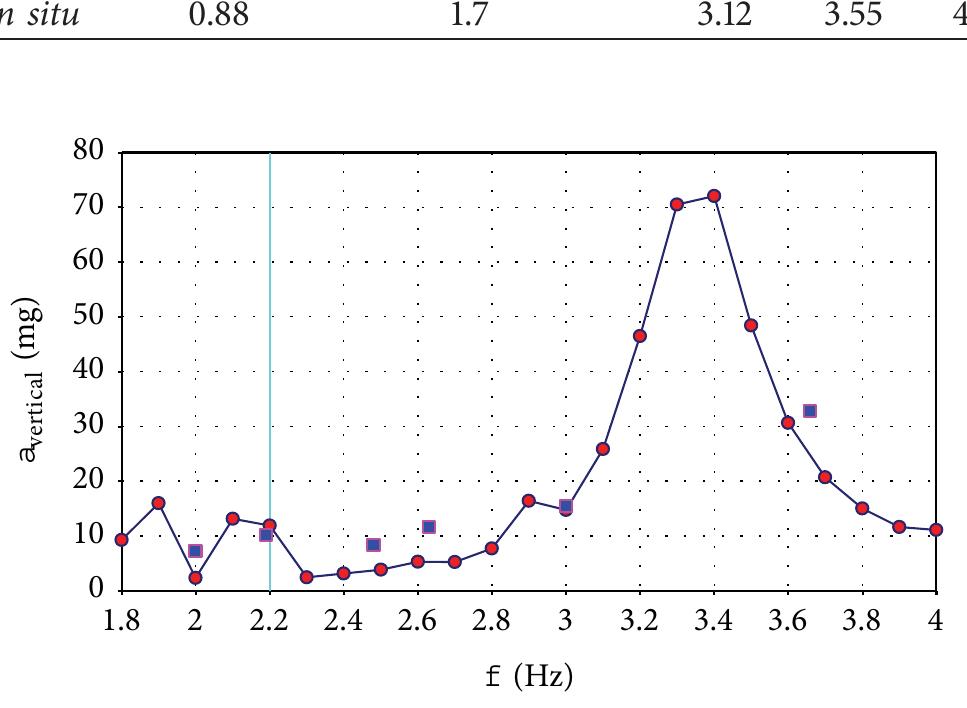
![TABLE 9: Comparison of frequencies (Hz) between the analytical model and measurements in situ. of lateral lock-in where feedback of lateral forces cancels out the positive action of damping of the structure, resulting in unbounded growth of response [34]:](https://figures.academia-assets.com/46494565/table_029.jpg)


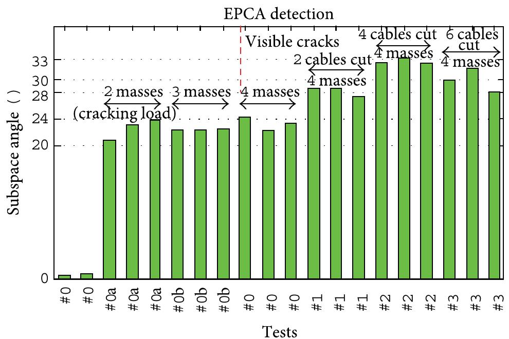
![The null subspace (NSA) and enhanced-PCA methoc (EPCA) proposed in [3, 4], respectively, are variant method: of the PCA method obtained by exploiting Hankel matrices of the dynamical system [8]. The data-driven block Hanke! matrix is defined in (3), where 2i is a user-defined numbe! of row blocks, each block contains m rows (number o: measurement sensors), and j is the number of column: (practically j = N — 2i+ 1). The Hankel matrix H, ,; consist: of 2im rows and is split into two equal parts of i block rows which represent past and future data, respectively. Comparec to the observation matrix X, the Hankel matrix is buil using time-lagged vibration signals and not instantaneou: representations of responses. This enables taking into accoun' time correlations between measurements when current date depend on past data. Therefore, the objective pursued here ir using block Hankel matrices rather than observation matrice: is to improve the sensitivity of the detection method: where the subscripts of H, 5, denote the subscript of the first and last element of the first column in the block Hankel matrix.](https://figures.academia-assets.com/46494565/figure_172.jpg)


![TABLE 1: Modal properties of the simulated 6-DOF system. been used also to validate an innovative automated OMA procedure in [9]. The selected real test cases are representative of modal identification problems typically encountered in civil engineering and characterized by different degree of difficulty. Reference modal parameters have been extracted from these records by well-established techniques, such as frequency domain decomposition (FDD) [31] and stochastic subspace identification (SSD) [1, 32], which have provided very consistent estimates. Figure 1: The benchmark 6-DOF system.](https://figures.academia-assets.com/46494565/table_039.jpg)

![TABLE 2: Test cases, modal identification results, and comparisons. SOBI-based automated OMA procedures for vibration-based SHM. It is worth pointing out that the possibility of automati- cally setting the analysis parameters without any preliminary calibration is a fundamental requirement for the development of automated OMA procedures. An effective control of computational efforts is possible by appropriate setting of t, taking into account that it negatively affects the accuracy of modal parameter estimates beyond the limit value of 1E — 4. Thus, the present paper provides a contribution towards the development of innovative automated OMA procedures able to satisfy widely accepted target criteria reported in the literature [6, 7, 9]. However, automated OMA based on SOBI is out of the scope of the paper.](https://figures.academia-assets.com/46494565/table_040.jpg)


![2.1. Representation in State Space Form. In order to obtain a nonlinear state space model, a rational function is used to write the aerodynamic forces in time domain. Jones in 1940 solved this problem using a rational function approximation to approximate unsteady aerodynamic loads for the typical section [24]. The expressions in (2) are rearranged ina matrix form and the nonlinear function f,) is introduced such that the stiffness is defined as a nonlinear structural stiffness matrix K,,; given by](https://figures.academia-assets.com/46494565/figure_199.jpg)
![where s is the Laplace variable, ),, is the number of lag terms, f; is the jth lag parameter (j = 1,...,m,g), and b is the aerodynamic semichord. In this paper Roger’s approach is used. This approxi- mation involves identifying every matrix Q; shown in (5) using a Least Square algorithm as proposed by Roger [29] and summarized in [30]. The approximation contains a polynomial part representing the forces on the typical section acting directly connected to the displacements u(t) and their first and second derivatives. Also, this equation has a rational part representing the influence of the wake acting on the section with a time delay. Consider](https://figures.academia-assets.com/46494565/figure_200.jpg)


![Ficure ll: Case 1: control surface rotation (|6] = 0.4° and V = 12.5 m/s). Ficure 10: Values of f,: actual versus computed using TS approach.](https://figures.academia-assets.com/46494565/figure_210.jpg)


![Ficure 14: Case: phase plan (|5| = 0.6° and V = 12.5 m/s). to 0.001 seconds. To compute the control gain, a column input matrix was used to represent an actuator applying force on the control surface (B,. = {0 0 1}7). Also, it was considered that the parameter g is equal to 1.0 for all cases. However, in particular for experimental applications where limitations exist on the actuator force, the parameter g can be conveniently chosen between ]0, 1[. functions, such that](https://figures.academia-assets.com/46494565/figure_213.jpg)


![and the linearised equations would remain coupled (unlike (5)) and consequently the gains in (6) would take a different form, as Clearly, there are a greater number of control gains in (8) than in (6), which means that there is more control flexibility, which might be used, for example, to assign the eigenvectors as well as the eigenvalues. This may be readily achieved using methods such as that presented in [11] and is illustrated through a numerical example later on.](https://figures.academia-assets.com/46494565/figure_223.jpg)


![A simplification in the matrix subscripts previously defined in [13] has been made here. The control force distribution matrix is given (as a function of air speed) by where f, and f, are control surface (flap) angles and T,,, is a control torque applied directly to the pylon-engine assembly. The nonlinear internal force is given by](https://figures.academia-assets.com/46494565/figure_227.jpg)
![The aeroservoelastic matrices are given in general terms in [13] and expressed here in terms of specific parameter values in consistent units (to three significant figures) as and the nonlinear time-domain response to initial conditions is produced at an air speed just above the flutter speed.](https://figures.academia-assets.com/46494565/figure_228.jpg)


![Control forces are applied to the wing-pylon-engine system by means of control surfaces. It is assumed in this work that two control surfaces (different from [14]) are available, the first (closest to the wing root) spanning 85% of the length of the wing and the second spanning the remaining length (the contribution of the control surfaces to the dynamics of the overall system is neglected). The widths of the first and second control surfaces are assumed to be 20% and 33.33% of the chord length, respectively. These particular dimensions have been chosen so as to optimise the distribution of work performed by each control surface. In addition to the ailerons, it is assumed that a separate actuator is available to apply a torque T,, directly on the engine rotational degree of freedom. The forcing vector is found to be](https://figures.academia-assets.com/46494565/figure_243.jpg)


![The use of the mass augmented objective function of (9) instead of (6) may lead to a compromise solution in which the system mass is minimized but the adjustment between the frequencies and mode shapes to their prescribed values may not be the best. Thus, the range constraints are added ((10)-(11)) so that the problem statement is now given by (9)- (13). Range constraints are used instead of strict equality constraints for two reasons. Firstly, satisfaction of equality of frequencies and mode shapes to their prescribed target values may not be possible depending on the design variables used for the synthesis [3]. Also, because the numerical optimiza- tion solution tends to be harder for strict equality constraints, even for the case where they are realizable. Here the multi- pliers p < 1 and q > 1 are parameters defining the ranges; for example, p = 1-6 and q = 1+, where 6 is adjusted during the optimization, departing from say 6 = 0.1, and closing the range with say 6 = 0.0001. Experience with simple cases now shows that good solutions can be obtained adjust- ing the ranges smoothly, by means of solving a sequential optimization with decreasing ranges such that in the ith opti- mization problem 6” = r 6°), where r < 1; for example, 0.1 < r < 0.5. Because of the new constraints we can choose the weights a; and b; to be null, so defining a cleaner mass- j only objective function. objective function and also range constraints for the frequen- cies eigenvalues and the MRQAs:](https://figures.academia-assets.com/46494565/figure_247.jpg)


![2.2. Modeling of Roughness. The random road surface rough- ness of the bridge can be described by a kind of zero-mean, real-valued, and stationary Gaussian process as [19] in which w, and w, are the lower and upper cut-off spatial frequencies, respectively. The power spectral density function S,(w,) can be expressed in terms of the spatial frequency w, of the road surface roughness as](https://figures.academia-assets.com/46494565/figure_263.jpg)


![Ficure 1: Destroyed reinforced concrete building by blast load [15]. structures. When a response of a building from blast load is considered, natural period of vibration of the structure is the vital parameter for a given explosion. Ductile elements made of steel and reinforced concrete absorb a lot of strain energy [3]. The effects of blast on reinforced concrete and steel structures have been widely studied by many researchers. To the knowledge of the author, the effects of corrosion with blast loads on reinforced concrete buildings have not been studied. Therefore, in this study, different blast load scenarios were performed for uncorroded and corroded reinforced concrete buildings to investigate the effect of blast loads with corrosion. Performance levels of the reinforced concrete buildings were obtained under the effect of blast loads. The impacts of the blast waves on the surface of the structural members were simulated.](https://figures.academia-assets.com/46494565/figure_270.jpg)


![FiGure 3: (a) Blast wave pressure-time graph. (b) Blast load and comparison [4].](https://figures.academia-assets.com/46494565/figure_273.jpg)
![Ficure 4: (a) Stress-strain relation of reinforced concrete [5]. (b) Stress-strain relation of steel bars [6].](https://figures.academia-assets.com/46494565/figure_274.jpg)


![To show the relation between (10) and (14), compute the estimate of the ith variable x; for a fixed mixture component k using (10). For clarity, the component index k is omitted. Consider 4. Damage Detection Using the mixture model for damage detection introduces an issue of residual scaling, because each class may have a differ- ent error variance (15). Therefore, the residual of each variable within each class is divided with the corresponding standard deviation, which is the square root of (15). Also the data dimensionality may be too high for statistical reliability (curse of dimensionality). Therefore, the first principal component scores [10] of residual (7) are used for damage detection. Control charts [ll] are used for damage detection. The control chart used in this study is the Shewhart chart [11], and the plotted variable is the subgroup mean of successive obser- vations. It is believed that the robustness of damage detection increases, because (1) additional variability due to environ- mental or operational influences can be removed, in this paper using a nonlinear model; (2) PCA is applied to the residuals avoiding the curse of dimensionality; and (3) con- trol charts utilize averaging for better statistical reliability.](https://figures.academia-assets.com/46494565/figure_299.jpg)