Journal of Dynamic Systems, Measurement, and Control

Moshe Shoham

Journal of Dynamic Systems, Measurement, and Control

Moshe Shoham

2000, Journal of Dynamic Systems, Measurement, and Control

visibility

…

description

247 pages

link

1 file

Abstract

Transactions of the ASME® Dynamic Systems and Control Division Technical Editor, A. GALIP ULSOY Past Editors, W. BOOK M. TOMIZUKA DM AUSLANDER JL SHEARER KN REID Y. TAKAHASHI MJ RABINS Associate Technical Editors, Y. CHAIT „2002… F. CONRAD „2001… E. FAHRENTHOLD „2001… S. FASSOIS „2001… Y. HURMUZLU „2001… R. LANGARI „2002… E. MISAWA „2002… S. NAIR „2001… N. OLGAC „2001… C. RAHN „2002… S. SIVASHANKAR „2002… J. TU „2002… P. VOULGARIS „2001… Book Review Editor A. GALIP ULSOY Executive ...

Figures (383)

Fig. 1 The rotational inverted pendulum system

Now, it is obvious that the right-hand side of the upper equation in system (34) does not depend on 6,. Following the approach of case 3, if the condition such that the right-hand side of the upper block in the motion equations would not depend on the time derivative of the state variable of the bottom block. Since x=3}—(C,/K,)6,, substitut- ing j' from system (31), yields

Table 1 Parameters of the rotational inverted pendulum system

Fig. 2 Hardware setup configuration of the pendulum system

Further, we will focus on the performance of the inverted pen- dulum system using our previously developed sliding mode con- trollers. Two case studies of the control objectives: case 1, stabi- lizing the pendulum at 6,=0 with @)=0, and case 2, stabilizing both the pendulum and the rotating base with respect to the equi- librium point 0)= 0,=0, will be presented.

Fig. 4 Simulation results by SMC for case 1: stabilizing the pendulum and it is fixed for other experimental results in the later figures. The control law utilizing a continuous approximation by a sinu- soidal function is designed as

Fig. 6 Experimental results by SMC: sloshing water (case 1) Fig. 5 Experimental results by SMC: no weight (case 1)

Fig. 7 Experimental results by SMC: metal bolts (case 1)

Fig. 8 Simulation results by SMC for case 2: stabilizing both the pendulum and the base

Fig. 9 Experimental results by SMC with small 6: no weight (case 2)

Fig. 10 Experimental results by SMC with larger 6: no weight (case 2)

Fig. 11 Experimental results by SMC: sloshing water (case 2)

Fig. 12 Experimental results by SMC: metal bolts (case 2)

Application of the Passivity Theorem. Using the notion of multipliers [2], the feedback systems shown in Fig. | are equiva- lent from the point of view of stability. The passivity theorem states that if G is passive and H is strictly passive then r eL,=yeL,. Using Lemma 1 and the passivity theorem, the original system is stable if either H= Y, TH or H= HY, is strictly passive. A possible design strategy would select H,,, a strictly Therefore G(s) is passive if and only if w<* When «= p*, the summation over the vibration modes vanishes (all vibration modes become unobservable) and the output p,,+=C,i7, becomes propor- tional to the rigid body modal rate. It 1s instructive to consider a small negative rate feedback u(t) = — ep,,. Using a simple eigen- value perturbation argument, it is readily shown that the closed- loop eigenvalues of each vibration mode are given by —€Y Cr lratja- All modes are stabilized when u<p* (Y, >0) and all of them are destabilized when p> (Y ,<0) as- suming controllability and observability, i.e., ¢.,#0.

Fig. 3 Torsional control system apparatus (reprinted courtesy of Educational Control Products)

The noncollocated degree of freedom is taken to be p,.= 03= 9 +[1 1]q, so that C,=1, C,=[11]. The collocated degree o' freedom is p.o= 9, and p,=wA,;+(1—) 4. If g-=6,, de) = 92.— 9, and g,.= 03— 9» are selected as gen- eralized coordinates and f(t) as the motor torque, the matrices defined in Eq. (2) are given by

Fig. 5 Parameter estimates (4*=0.973, 4=0.96)

Fig. 6 Tracking errors and parameter estimates (u*=0.567, p=0.55) Table 2 Measured values of 4, at stability-boundary

pole locations p, are defined by p.= Bp, (see Fig. 1), or if dis- crete time control is used p.=e P47, where AT is the sampling time. This way of scaling maintains the damping of the poles, while > changing the speed of the response.

Fig. 2 Scaling design for PD control of a double integrator plant From Fig. 2 it is clear that the performance can be improved by increasing 6 outside the interval (0,8);,) where the control does

Theorem 4.1 is illustrated schematically for a second order ex- ample in Fig. 3. Theorem 4.1 does not say anything about how to obtain the matrix P. Any choice of P that satisfies Eq. (8) for a =1 can be used; it then follows that there exists an ayin<1.

Table 1 Comparison of design methods, full state feedback of a number of numerical optimization techniques can be used to minimize S(P,) for a fixed 8, and thereby find a P such that

Fig. 4 Simulation results for x(0)=[0 0.71 0.71]? and B=0.79, 2.29, and 3.23 conditions is a limited number of points in state space, it is pos- sible to obtain 6,,, quite accurately. The accuracy is determined by the size of the change in the parameter 8 used when searching for Boot -

with plant state x e %", integral state x; = 9%, and controlled output ze. The AW is shown in block diagram form in Fig. 5, where q denotes the unit delay operator. This structure is very typical for many AW methods; what is special about this method is the spe- cial choice of the AW gain that results in the integral state becom- ing a function of the state x during saturation.

Table 2 Comparison of design methods, full state feedback plus integral control

Fig. 10 Experimental and simulation result for full state feed- back control 9 Conclusions Finally, the stability based method is applied to the case of full state feedback plus integral control for the same plant as in the previous example. In this case it turns out that the limiting factor is not the saturation, but the unmodeled dynamics. This means that the design parameter £ has to be limited to avoid exiting the

Fig. 2 Schematic of a multilimbed robot Fig. 1 Simplified Cartesian computed torque (SSCT) control

ee ee ee ee eee eee Oe eee ee The SCCT control scheme is applied to a multilimbed robot, such as the robot shown in Fig. 2 as follows. The various limbs of the robot are viewed as manipulators, each doing a different task. Some limbs support and position the robot body, some carry and manipulate objects, and some apply forces to the environment. Each limb is under SCCT control and the desired reference inputs are appropriately selected for its task. For example, for free limbs that move in space, the controller shown in Figure 1 can be ap- plied with X,,, and X,,, being the desired and actual position/ orientation of the tip of the limb with respect to the body. For limbs that are in contact with the ground and are used to position the body, the variant of SCCT control shown in Fig. 3 can be used. In this case, Xq., and X,,; are the body’s desired and actual

Table 1 Model parameters of LIBRA’s joints

Fig. 3 Block diagram for the control of a multilimbed robot

5 Experimental Results of SCCT Control Applied to One Limb

Fig. 6 Comparison of experimental system and simplified model Experiments were performed to compare the Jacobian transpose and SCCT control schemes for simple endpoint under position control of one limb. Figure 7 compares the two controllers for a step input. The tip of the limb is commanded to move 2 cm in the Y direction: from point A to point B in the figure. The SCCT controller is able to hold the limb’s X position essentially constant

Fig. 7 Step response of two Cartesian controllers

Fig. 8 Experimental path tracking of the two Cartesian con- trollers

Fig. 9 Stiffness selection in Cartesian space

Fig. 10 One complete step in a LIBRA climbing gait

Note that, in the basic backstepping procedure, at Step n one determines the actual control as aS Eee ee ee eee lee ee To apply the second order variable structure control strategy within the backstepping framework, the sliding manifold

The two dynamical Eqs. (12) complete the transformation from the state [x1(1),....x,(D ]7 to the state [21 (1),.--5Z,—1(t),e1(t),e2(t)]’.. With implicit symbol defini- tions, system (12) can be rewritten as The idea is now that of steering both e,(ft) and the unmeasurable (ft) to zero (to attain the sliding regime on S(t)=S(t)=0) ina finite time, that is, a second order sliding mode control problem has to be solved. In Bartolini et al. [26], it has been proved that, by analogy to the well-known solution to the time optimal control problem, the control u(t) can be chosen as a bang-bang control switching be- tween two values — Uy, and +Uy,,. The classical switching logic for a double integrator (H(e,(t), e2(t))=0, Bj, =B,=1) is

J, J ace the load and motor inertias, F,,F,, are the load and motor damping constants, k is the joint stiffness, and u is the input torque applied to the motor shaft. Assume that J,,=J,,(x) as it happens in practical situation in which the motor is driven by the input voltage through a nonlinear element the characteristic of which is a function of the system state. System (25) can be rewrit- ten as

VxeB,, V@eBj, where B, and Bg are neighborhood of the equilibrium point in the x-space and 6-space, respectively. B(x) has been replaced by B(x,v), that is a linear function in the v variable (it represents the dependence from the @ parameters in Eq. (2), here is substituted with its estimate as it appears as coef- ficient in the expression of u).

Fig. 2 Output trajectory in the proposed procedure

Fig. 5 S trajectory in the proposed procedure

Fig. 4 u trajectory in the proposed procedure

Fig. 6 0 trajectories in the proposed procedure

where q, g, and g are, respectively, the n <1 joint position, ve- locity, and acceleration vectors, u represents the n X 1 torque vec- tor generated by actuators, M(q) is the symmetric positive defi- nite generalized inertia matrix, C(q,q) is the force (torque) vector resulting from Coriolis and centripetal accelerations, G(q) is the generalized gravitational force vector, and d(q,q) denotes the dis- turbance. Define a 2n-dimensional state vector x as

This completes the proof of the following theorem: ee - Theorem: For a robot model Eq. (1) subject to sliding mode based repetitive learning control, which is accounted for by Eq. (19), the sliding surface S and the tracking error e are uniformly bounded if both gain matrices K and Q in the reaching law are adequately chosen. Furthermore, having learned a number of cycles, the ultimate tracking error e is bounded by [t is always feasible to adequately choose K, A, T’, and oy such that R is positive definite. Therefore, one can prescribe values of positive constants o,, 7,, and og to satisfy

Fig. 1 Schematic diagram of direct-drive robot As shown in Fig. 1, this study constructs a three-axis R— 6 —Z direct-drive robot manipulator, where the first link is driven by a NSK Megatorque motor [14], the second by a NSK Mega- thrust motor, and the third by an electrothrust motor together with ball screw.

The speed and acceleration profiles of the end-effector are pre- scribed as shown in Figs. 4(a) and 4(b), respectively. Figure 5 depicts a spatial circular trajectory to be tracked. In addition, a planar square trajectory on the X—Z plane, will also be carried out in experiments. Figure 6 depicts the control block diagram. To implement the present method, Eqs. (11), (13), and (14) are re- written to become the discretized form:

Fig. 6 Control block diagram of the present method

Fig. 4 (a) Speed profile of end-effector and (b) corresponding acceleration profile

Fig. 8 Position errors in Z-axis using (a) sliding mode control and (b) the present method Fig. 9 Sliding variables in R-axis using (a) sliding mode con- trol and (b) the present method (1) Spatial Circular Trajectory Tracking. In contrast to Fig. 8(a), tracking errors in Fig. 8(b) progressively reduce to a smaller

Fig. 13 Tracking result of the first time learning in X-Z plane Fig. 10 Tracking result of the first time learning in Y-Z plane

Fig. 12 Position errors in Z-axis using (a) sliding mode con- trol and (b) the present method Fig. 11 Tracking result of the fifth time learning in Y-Z plane

Fig. 14 Tracking result of the fifth time learning in X-Z plane

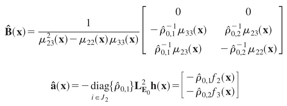
and where use was made of the definition of E(x) and of the fact that po;#0, ie J,. Next consider the matrices [[9(x) Ao(x)] and [T,(x) A,(x)] defined as

We are now able to establish the following theorem. Eee eS ee ee eee ee Theorem 4.1. The DRLD problem via the restricted state feed- back law (2.3) is solvable if and only if there exists a set of nonnegative integers {Y1,s,-.-,Yp,s+ Such that the following condi- tions simultaneously hold:

Example 5.1. Consider the nonsquare nonlinear analytic system of the form (2.1) with whose input-output description consists of the following set of differential equations: In order to demonstrate the efficiency of our approach, the fol- lowing illustrative examples are presented:

Example 5.2. Consider the nonsquare nonlinear analytic system of the form (2.1) with Finally, as it can be easily checked, for the choices (y\,;,¥2,) =(0,1) or (1,0) or (1,1) or (0,2) or (2,0), Theorem 4.1 cannot be satisfied.

Hence, the appropriate restricted state feedback is characterized by where fo; .i€ J, are arbitrary nonzero real parameters. It is easy to see that, application of the above restricted state feedback to the system at hand yields an I/O linearized and simultaneously decou- pled and disturbance localized system, whose input-output de- scription has the form

Therefore, the appropriate restricted state feedback is given by where fo;, 1¢Jy are arbitrary nonzero real parameters. The closed-loop system has the input-output description It can be easily checked that for the remaining choices of the pair (Vis+¥2s), Theorem 4.1 cannot be satisfied.

where f9;,1€J2 are arbitrary nonzero real parameters. The closed-loop system has the input-output description Therefore, the appropriate restricted state feedback is given by

Space station dynamics: Journal of Dynamic Systems, Measurement, and Conirol NE Rg OE Ley © Example 5.4. The nonlinear equations of motion of the space station rotating in circular orbit with constant orbital rate, in terms of components along the body-fixed control axes can be written as [28]

Assuming a constant orbital rate and differentiating (5.5), we obtain Solving (5.3) with respect to the vector [w, w w3]|, we obtait

where, g;,92.q3 are the body-axis components of the CMG mo- mentum. Pa a Sy aa ee Oe ee Ee 2) 317T .— .44¢.°. Attitude kinematics (2-3-1 body-axis sequence):

Therefore, Theorem 4.1 is satisfied for (y1,5,¥2,;)=(0,0) and the problem is solvable. Moreover, we have

Fig. 1 Sensitivity curves relative to normalized frequency for ZV, ZVD, and El input shapers (@mogei=1 rad/sec, Cmoget= 0-01, ty=4a sec).

Fig. 2 Shaper lengths for optimal shaper designs assuming uniform (top) and Gaussian (bottom) variation in the natural frequency. The ZVD and El shaper lengths (which are equal) are also shown for comparison.

Fig. 3 Comparison of the 5 percent insensitivity W; levels as- suming for optimal shaper designs uniform (top) and Gaussian (bottom) variation in the natural frequency.

Fig. 4 Comparison of the expected residual vibration (J) assuming for optimal shaper designs uniform (left) and Gaussian (right) variation in the natural frequency. For smaller parameter uncertainties, the ZVD is more optimal; and as the parameter uncertainty increases, the El shaper becomes closer to optimal.

Fig. 5 Comparison of the magnitude of shaper zeros assuming for optimal shaper designs uniform (left) and Gaussian (right) variation in the natural frequency.

Fig. 6 Shaper length of minimal expected residual vibration shapers assuming uniform and Gaussian variation in both fre- quency and damping. For lightly damped systems, optimal shapers yield shorter shaper lengths than those obtained from traditional ZVD and El shaper designs.

Fig. 7 Expected residual vibration (J) assuming for optimal shaper designs uniform (top) and Gaussian (bottom) variation in both frequency and damping. Optimal shapers yield lower expected residual vibration than those of ZVD and EI designs.

Fig. 9 Shaper lengths for different uniform frequency uncer- tainties. The optimal shapers yield shorter shaper lengths com- pared with traditional ZV shaper designs. As in the comparison of three-impulse optimal shapers and tra- ditional ZVD and EI shapers, we see that the optimal shapers lead to faster maneuvers while yielding lower levels of expected re- sidual vibration, as shown in Figs. 9 and 10. A uniform frequency

Fig. 8 Angle deviation of optimal shaper zeros from system poles for uniform (top) and Gaussian (bottom) variation in fre- quency and damping. The angle deviation is negative for the optimal shaper zeros meaning that their location is shifted to- ward a line of lower damping.

Fig. 10 Expected residual vibration for different uniform un- certainty ranges in frequency. The optimal shapers yield lower expected residual vibration compared with the traditional ZV shaper designs. uncertainty size of 0.1 means w is uniformly distributed from 0.9@ moder tO 1.1@mode, and similarly for other frequency uncer- tainty sizes.

Fig. 2 Material deposition from mass source to the molten globule

Fig. 3 Numerical simulation of thermal material transfer

Fig. 4 Molten globule modeling through a spherical lens primitive However, when solidification occurs under nonequilibrium con- ditions, i.e., during surface oscillation, or under the influence of the mass and/or heat source and a shielding gas stream, the geom- etry of the elementary deposition field deviates from the simple shape of Fig. 4. The same is true when material is deposited on a nonflat substrate (i.e., adjacent to previously laid beads) or not horizontal to gravity. Figure 5(a) shows such a unit deposition distribution identified in gas metal arc welding (GMAW) with a consumable stainless steel electrode over a similar substrate. Fig- ure 5(b) illustrates how such a deposition field Z can be composed by a number n of elementary spherical lens primitives Z;, each defined by parameters u;,U;,W;.1;:

Fig. 5 Material deposition field Z in GMAW: (a) composite deposition distribution Z; (b) decomposition into spherical primitives > Z;

Fig. 6 Distributed-parameter model of surface geometry z by superposition of deposition fields Z Equation (9) updates the time-dependent, arbitrary-shaped deposition distribution Z, by assessing the deviation field «=z —z between the actual measurements z and the predicted geom- etry z. This distributed-parameter identification can be performed in real time, by periodic adjustment of Z every Dt, with only a limited number of local geometry data at locations (y,y) needed to

Equation (8) actually represents a locally linearized, time-varying (LTV) description of the nonlinear phenomena composing mate- rial deposition, as already discussed. The nonstationary lineariza- tion and the respective parameter uncertainty of the mass transfer nonlinearities are reflected in the time variation of the deposition distribution Z. Thus, rather than anticipating an exacting model of these complex effects on physical grounds, an approximation of the composite deposition field Z Eq. (5) will be updated through experimental identification of its parameters (u;,v;,w;.r;). If laboratory data on a part of the surface geometry z(x,y;f) are obtained over a time period Dt, the deposition field Z can be identified by incremental deconvolution of Eq. (8), based on the applied material feed F(X,Y;7) from the mass source along its motion:

In principle, given geometric measurements z at 4n locations (y,y) on the part surface, and the respective predictions z of the deposition model from Eq. (8), the resulting deviation values can be used in Eq. (10) to form a linear system of 4n equations, to be solved for the deposition parameter changes (Du; ,Dv;,Dw;,Dr;),i=1...n. Notice that in order to obtain such a well-conditioned system of equations for robust parameter identification, sufficiently rich data must be obtained at respective 4n positions (y,), located close and scattered around the current material deposition region. In the vicinity of the mass source (X,Y), however, real-time measurements, e.g., by mechanical pro- filometry or optical scanner sensing, are technically problematic because of the material deposition interference with the sensor. Moreover, the precision of the geometry model is challenged by the variable source influences, due to the dominating surface ten- sion assumption. For this reason, in-process geometry measure- ments at m locations are conducted on the solidified surface at a safe distance behind the mass source, as explained below. On the basis of these m measurements, the 4n deposition parameter changes are evaluated by a least-squares identification technique (Astrom and Wittenmark [24]). This method minimizes a qua- dratic index *e(t) of the deposition error ¢ values at the m mea- surement locations, analogous to that of Eq. (6). The resulting corrections Du;,Dv;,Dw;,Dr;,i=1...n, are subsequently used every time period Dt to update the deposition field param- eters u;,U;,W;,r;, to their new values u;+Du;,v;+Dv;,w; +Dw;,,r;+Dr;. identify the parameters (u; ,v; ,w;,7;) of the composite deposition field approximation Z, Eq. (5). For this purpose, Eq. (9) can be rewritten over the full process duration ¢, as a linearized expres- sion of the deviation field ¢ sensitivity on the parameter variations Dy. Dn. Dw. Dr. j=1.. 2 -n-

Fig. 7 Experimental station for GMAW thermal material depo- sition with laser stripe optical scanner The geometry of the deposited material profile is measured in- process, along a line segment across the direction of motion and trailing behind the mass source (Fig. 8). This is obtained by a 3D optical scanning system based on a sweeping laser stripe. It con- sists of a 20 mW laser diode, which through a cylindrical lens projects a bright light stripe on the prototype surface. The laser stripe is shed across the deposited bead and it follows the GMAW torch at a distance I=25.4mm, separated by an incandescent cloth partition to minimize light interference from the arc. The deflections of this line as it sweeps the deposited material reflect the geometric profile of the latter, and are monitored by an optical CCD camera with band-pass filtering at the laser wavelength (680 nm). The optical image is monitored in real time by the system computer, through a frame grabber and image processing soft- ware, and is also recorded in standard video format for off-line analysis. This software includes algorithms for the CCD camera elevation angle correction and gray-scale interpolation of the height z at the m measurement locations O; ,i=1...m along the laser stripe, with an accuracy of 0.1 mm. Note that the distance I

Fig.8 Arrangement of laser stripe scanner for geometric mea- surement of bead profiles

Fig. 9 Open-loop bead width and height responses to torch velocity changes: zig-zag line: experimental measurements; long-dashed line: analytic model predictions

Fig. 10 Block diagram of distributed parameter geometry controller for material deposition

Fig.1 Stribeck curve. The duty parameter is defined as p;v/F, where yp; is the lubricant viscosity, v is the sliding velocity, anc F,, is the normal force per unit contact area.

Fig. 2 A simplified condition of polymer-to-metal contact with lubricant. m, is the average separation between the polymer and metal surfaces with maximum My and minimum M,,, A, is the local deformation on the polymer surface with maximum Ay and minimum 4A,, .

Fig. 3 Schematic of a hydraulic actuator, the seals are all made of polymers and both sides of the piston are filled with hydraulic fluid. Lubricated polymer friction exists at all seal-to- metal contacts.

Fig. 4 Comparison of the deterministic model (dashed line) and the measured data (solid line)

Fig. 5 Comparison of the overall stochastic model (dashed line) and the measured data (solid line)

Fig. 6 The estimated normalized autocorrelation function of the prediction error of the stochastic model. The two parallel dashed lines denote 95% confidence interval.

Fig. 8 The estimated normalized autocorrelation function of the prediction error of the extended Kalman filter after 1 hour and 32 minutes of reciprocating sliding. The two parallel dashed lines denote 95% confidence interval. Fig. 7 A close-up of the extended Kalman filter’s estimates (marked by *) and the measured data (solid line) after 1 hour and 32 minutes of reciprocating sliding

Fig. 9 A close-up of the extended Kalman filter’s estimates (marked by *) and the measured data (solid line) after 8 hours of reciprocating sliding

5 Conclusion Fig. 12 The trajectory of parameter a, after 8 hours of recip- rocating sliding

Fig. 11 The trajectory of parameter a, after 1 hour and 32 min- utes of reciprocating sliding Fig. 10 The estimated normalized autocorrelation function of the prediction error of the extended Kalman filter after 8 hours of reciprocating sliding. The two parallel dashed lines denote 95% confidence interval.

Fig. 13 The trajectory of parameter G3 after 1 hour and 32 minutes of reciprocating sliding

Fig. 14 The trajectory of parameter G3 after 8 hours of recip- rocating sliding

Fig. 2 Flow chart showing the battery of tests for identifica- tion and characterization of underlying process dynamics Fig.1 Poincare section plots of force and vibration signals—collected at cutting speed V=130 ft/min, feed f=0.0088 in./rev—capturing the variations in machining dynamics with flank wear. Fresh, partially worn and fully worn refer, respectively, to h,=0.000, 0.0060, and 0.0175 in.

Fig. 3 Methodology of fractal estimation consisting of an offline training phase and an online estimation phase 3.1 Experimentation. The experiments were conducted on a 20 HP LeBlond heavy duty lathe. The workpieces were made of 36in.x é7in. SAE 6150 Cr-V steel, and the tool inserts were uncoated carbide grade K68 with geometric specification SPG- 422. Three different online sensors were used—(i) a three-axis Kistler Z3392/b piezoelectric dynamometer, placed underneath

Fig. 4 Design of experiments: Solid and dashed outlines of circle indicate whether that the exemplar patterns corresponding to that design point are used for training or testing

Fig. 5 Representative plots showing (a) the variation of aver- age fractal dimension with d; for two experimental runs con- ducted using a fresh tool: V=160 ft/min, f=0.0136 in/rev. (b) the effect of signal separation on the fractal dimension esti- mates: — corresponds to the separated signal, and —--—-—-— corresponds to the nonseparated signal. As a result of signal separation, the change of slope of the graph becomes more pronounced. This reduces the uncertainty in deciding the linear portion of the graph thus rendering the computation of the slope of the linear portion of the graph, and hence the fractal dimension estimates more accurate.

Fig. 6 Architecture of the recurrent neural network Table 1 Sample input patterns Table 2. Neural network training details

Fig. 7 Influence of time of cutting, and hence the extent of flank wear, on the estimation error

Fig. 8 (a) Comparison of interpolates of the flank wear esti- mates (— — —) and the actual measured flank wear (—). The experiment was conducted at V=160 ft/min and f=0.0136 in/rev. (b) An empirical q—q plot showing the equivalence of the distributions of the estimation errors corresponding to the exemplar patterns used for training the neural network, and those corresponding to the testing patterns.

Fig. 1 Flowchart for the FRF-based identification scheme The overall procedure for joint parameter identification is sche- matically depicted in Fig. 1. The identification of joint parameters requires an FEM model of the structure without joints and experi- mental measurement of FRF’s at a few selected points. FRF’s at necessary points, particularly at joint locations, are estimated by using an indirect estimation technique described in Sec. 2.1. The joint parameter identification procedure is described in Sec. 2.2.

and W;(w) is a weighting function to take into account the reli- ability of identification with respect to frequency. Assuming, without loss of generality, the bearings have con- stant stiffness and damping coefficients over a certain range of frequency, it will be useful to make use of the following weighted average for the bearing parameters, i.e., Since the above identification formula has a linear relationship with the indirectly estimated FRF’s, it may be useful to use //(w) as the weighting function for Eqs. (11) and (12) or for selecting the frequency range appropriate for identification. In addition, magnitudes of the FRF’s involved in the matrices can reveal the relative importance of the results as a function of frequency. Therefore, the magnitudes of some FRF’s related to the identifi-

Fig. 2 Configuration of the high speed spindle with cutter and toolholder 3.1.1 Experimental Setup and Measurement of FRF’s. The spindle system consists of a 6 in. cutter connected to the spindle by a size 50 taper toolholder. The spindle is a horizontally mounted high speed spindle with the maximum rotational speed of 10,000 rpm and is driven by a 100 HP DC motor through a 3 in. wide belt. The spindle is equipped with two sets of tapered

Fig. 3 Experiment 1: (a) index functions; (b) measured FRF at the rear end; (c) measured FRF at the front 3.1.2 Identification of Stiffness Coefficients. The selection of the frequency range for identification is a two step process. The first selection is based on a broader range of frequency and is used in the identification program. This initial range is determined by cluding the majority of the main lobes of the frequency re- sponse. For experiment 1, this range was chosen to be from 650 to 300 Hz based on Fig. 3 (b-c). The identification produces an identified stiffness value at each frequency in the selected fre- quency range. The second frequency range is determined by a

Table 2 Identified stiffness of the high speed mill spindle combination of the index functions and the magnitude of the FRE. Once the second frequency range is determined, a weighted aver- age based upon the index functions provides a single, averaged stiffness value for each bearing to be identified. The second quency range selected for experiment 1 was 760 to 790 Hz d fre- eter- mined from Fig. 3 (a—c). To verify that the measured FRF’s are acceptable, coherence functions were obtained. The coherence functions for experiments 1 and 4 are shown in Fig. 4. Since experiments 5 through 7 were conducted with the changed p hysi- cal system, the first frequency range selected for the identification was changed accordingly to include the majority of the main lobe measured for each experiment. The second frequency range se- lected corresponded to the higher index values associated with the main lobe.

Fig. 5 Comparison of measured FRF’s and estimated FRF’s with transverse damping for experiment 2: (a) rear; (b) front The stiffness values for all the experiments are provided in Table 2. Since the front and rear bearings used in this milling machine are two different types, the stiffness parameters are not

Fig. 4 Coherence functions in FRF measurement: (a) experi- ment 1, front; (b) experiment 1, rear; (c) experiment 4, front; (d) experiment 4, rear

Fig. 7 Comparison of measured FRF’s and estimated FRF’s with transverse and tilting damping for experiment 2: (a) rear; (b) front Fig. 6 First three mode shapes of the horizontal mill spindle

3.1.4 Tilting Damping Identification. Observation of experi- mental results shows that the third mode is overdamped. How- ever, since the bearings (located at 0.2083 and 0.5458 m) are near the nodal points for the third mode as shown in Fig. 6, transverse damping alone will not be able to correctly model the damping

Table 3 Identified damping of the high speed mill spindle

Fig. 8 Comparison of measured FRF’s and estimated FRF’s with transverse and tilting damping for experiment 1: (a) rear; (b) front

Fig. 10 MAZAK spindle experiment: (a) index functions; (b) measured FRF on the toolholder directly below the spindle; (c) measured FRF at the tip of the extension tool

Table 4 Theoretical and identified stiffness for the MAZAK spindle

Table 5 Natural frequency prediction and validation for the MAZAK spindle Nomenclature

In order to rearrange the system matrices into measured and un- measured DOFs, an identity relation is introduced into Eq. (A2)

Fig. 1 Probe type sensor and CCS: (a) using four probe sen- sor; (b) using the CCS

Fig. 4 Capacitance at the eccentric rotor position Wiodeling OF the KouNndness Krrors Of the Kotor and the Sensor. The roundness error of the rotor deteriorates the distor- tion of the line, as shown in Fig. 4. If the roundness error is h (function of 6), the small variation Au from the nominal straight u,, can be expressed as Fig. 3 Capacitance at the concentric rotor position

Fig.5 The effect of the sensor size ¢ on the error amplification factor e,,/h,, with various odd harmonic numbers of m

Fig. 7 Test rotors with harmonic roundness errors: (a) rotor 1; (b) rotor 2

Fig. 6 Measurement errors of two probe sensors, four probe sensors, and the CCS (dia. of rotor 50 mm gap between sensor and rotor 0.5 mm magnitude of roundness error 0.001 mm ra- dius of revolution 0.003 mm)

Fig. 8 Magnitudes of harmonic errors of each testing rotor

Fig. 10 Simulation of measuring orbits of test rotors with vari- ous sensor types (dia. of test rotor 50 mm depth of harmonic error 0.05 mm, radii of revolution 0.02 mm, and 0.03 mm). (a) Rotor 1 with third harmonic error; (b) rotor 2 with fourth har- monic error. Two test rotors are shown in Fig. 7 and the experimental setup is built as shown in Fig. 9(a). The experimental setup consists of speed controlled DC motor, hydrostatic bearing, oil-less bearing, spindle with test rotor and sensor housing with four probe sensors, and the CCS. The probe sensor used is a capacitive sensor, PX405HA manufactured by LION PRECISION. The photo of the

Fig.9 Experimental setup: (a) schematics; (b) sensor housing

Fig. 11 Experiments of measuring orbits of test rotors with various sensor types (dia. of test rotor 50 mm, depth of har- monic error 0.05 mm, radii of revolution 0.02 mm and 0.03 mm). (a) Rotor 1 with third harmonic error; (b) rotor 2 with fourth harmonic error.

Fig. 13 Mounting errors of probe sensor small rotation of the sensor coordinates from the reference coor- dinates and by not heading toward the reference origin. As the latter exists at =O, the effect of this error is expressed as small distortion of the sensor.

Fig. 12 Mounting errors of the CCS: (a) misalignment; (b) angle error

Fig. 1 The unperturbed system in the roll manifold

Fig.5 Roll dynamics with parameter variations under different controllers: nonlinear feedback (solid), linear feedback (dash— dot), and open loop (dashed) Without parameter variations, the peak control effort using non- linear feedback control is uy,,,=1.45 for IC1 and u,,,,=2.24 for IC2, and for the linear feedback control that value is uy,,,=3.40 for IC2. With parameter variations under nonlinear control, upax =3.88 for IC1 and w,,,,=8.05 for IC2. These peak control efforts usually occur during the initial transient period and settle down to smaller levels soon after. The peak control effort required for the cases with parameter variations is somewhat larger, as expected. It can be reduced by tuning down the control parameters, however, at the expense of roll reduction performance.

Fig. 4 Roll dynamics without parameter variations under dif- ferent controllers: nonlinear feedback (solid), linear feedback (dash—dot), and open loop (dashed)

Fig. 1 The proposed ER damper: (a) Schematic configuration; (b) photograph Here E is the electric field. The a and @ are intrinsic values of the ER fluid to be experimentally determined. In this study, for the ER fluid, the commercial one (Rheobay, TP Al 3565) is used and its yield stress at room temperature is reported by 591E!“? Pa [7]. Here the unit of E is kV/mm. It is herein noted that the Bingham model of the ER fluid [8] is adopted for the derivation of Eqs. (1) and (3).

Fig. 2 Damping force versus piston velocity at various electric fields: (a) measured; (b) simulated

Fig. 4 Bond graph model of the ER suspension system Fig. 3 Mechanical model of the full-car ER suspension system

replacing the sign function by the saturation function with appro- priated boundary layer thickness ¢; for (i= 1,2,3,4). The control- ler u given by Eq. (13) is designed in an active actuating manner. However, the ER damper is a semiactive actuator. Thus, the con- trol input force should be applied to the ER suspension system according to the following actuating condition. In this study, HILS is undertaken to evaluate the performance of the full-car ER suspension system. The configuration of the proposed HILS is schematically shown in Fig. 5. The HILS is divided into three parts: interface, hardware, and software. The interface part is composed of computer (IBM, Pentium-133 MHz) on which DSP board (Mtt, TMS320C31) is mounted. To drive the DSP board in real time, Matlab® program with Simulink® tool- box is used and its looping time is chosen by 0.9 ms. The hard- ware part is composed of the ER damper, high voltage amplifie (Trek 10/10A), and hydraulic damper tester (hydraulic power unit). The software part consists of the theoretical model for the full-car ER suspension system and control algorithm programmed n the computer. The photograph of each component for the HILS is shown in Fig. 6. As a first step, the computer simulation for the full-car ER suspension system is performed with initial value. This computer simulation is incorporated with the hydraulic damper tester which applies the displacement (suspension travel) to the ER damper according to the demand signal obtained from the computer. It is also connected to the high voltage amplifie which applies control electric field determined from control algo- emi

Table 1 Parameters of the full-car ER suspension system rithm to the ER damper. Then, the damping force of the ER damper is measured from the hydraulic damper tester and the measured damping force is fed back into the computer simulation. In short, the computer simultaneously runs both the hydraulic damper tester and high voltage amplifier during simulation loop, and the computer simulation is performed based on the measured data. In this study, the ER damper at rear right side is chosen for the HILS by considering the capacity of the hydraulic damper tester. (=0.856 m/s). The second type of road excitation, normally used to evaluate the frequency response, is a stationary random process [14] with zero mean described by

Fig. 7 Trajectory tracking performance of the hydraulic damper tester: (a) bump and (b) random excitation Here w,=27V/D, z,(=0.035 m) is the half of the bump height, D(=0.8 m) is the width of the bump, D,,,(=2.4 m) is the wheel base which is defined as the distance between the front wheel and the rear one, and V is the vehicle velocity. In the bump excitation, the vehicle travels the bump with constant velocity of 3.08 km/h

Fig. 8 Controlled responses of the ER suspension system for bump excitation: (a) without and (b) with parameter perturba- tions We first investigate the tracking performance of the hydraulic damper tester during simulation loop prior to implementing the HILS. Figure 7 presents suspension travel tracking performance

Fig. 9 Controlled frequency responses of the ER suspension system for random excitation: (a) without and (b) with param- eter perturbations

Let us for simplicity define the time dependent gas velocity of the inlet port, v, (x,,)=v,.. The inlet port gas velocity, v,, can be approximated (Broome [16], Moraal et al. [13]) by the solution to a second order forced differential equation with known initial values:

where, r.=(2/(y+1))”~! is the critical pressure ratio. Mh SSeS ee ee ae ts Fore aR: TSE Fs arses a I SCN eR a ae Sea ae The above expression is simplified by taking into account that for camless unthrottled operation the intake manifold pressure is almost equal to the ambient pressure py= 10° Pa. In addition, we consider 7; =T,=T=316°K, R=287 J/kgk, y=1.4 and that typical operation results in limited backflow through the orifice (p,/p2=1.1). The flow equation

The approximation simplifies significantly the computation an results in fast execution of the simulations. Thus, the flow throug! the throttle body, mg, and the intake valve, m,, are written as where, A,=A,,k (m7) is the effective flow area function for the valve normalized at sonic conditions and constant temperature, and d is defined:

Fig. 1 Camless valvetrain controller (‘inner loop”) and cam- less engine controller (‘“‘outer loop’’)

Fig. 3 Intake valve profiles for different speeds Fig. 2 Electro-hydraulic camless (dashed), simplified camless (solid), and conventional (dotted) intake valve profiles 3 Performance Variables

Fig. 4 Engine breathing characteristics of a 4-cylinder engine at an engine speed of 1500 rpm

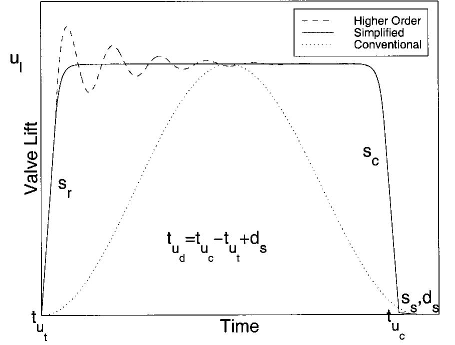
Fig. 6 Model (dashed line) versus experimental data (solid line) at 1500 rpm The model described in this paper was evaluated using experi- mental data for a 4-cylinder engine (Moraal et al. [13]) during wide open throttle operation. The valves of the experimental en- gine are cam-driven, therefore, the intake valve profile is the con- ventional sinusoidal profile with the following specifications: (i)

Fig. 5 Cylinder P-V diagrams that demonstrate the pumping loss in a throttled and a camless unthrottled engine (lift profiles are also shown)

Fig. 8 Model (dashed line) versus experimental data (solid line) at 4000 rpm In Figs. 6, 7, and 8 we compare the model with the actual engine data for wide open throttle (f in Eq. (15) is fixed to 90 deg) and engine speeds of 1500, 3000, and 4000 rpm, respec- tively. The manifold and cylinder pressures are plotted for the model (dashed curve) and the experimental engine (solid curve). The model Helmholtz resonator parameters were determined as w,=27*176, €,=0.005 for an engine speed of 1500 rpm, and w,=27*190, €,=0.15 for engine speed of 3000 and 4000 rpm. These values are similar to the ones identified in (Moraal et al. [17]).

Fig. 7 Model (dashed line) versus experimental data (solid line) at 3000 rpm

Note that the model captures most of the dynamic effects. Moreover, the model predicts rather accurately the integral quan- tities, namely, the cylinder air charge and pumping losses, which are overall measures of the engine performance over the induction stroke. The comparison of predicted cylinder air charge (77) and pumping loss (£) versus the actual data cylinder air charge (m) and the pumping loss (£) follows: The maximum error in air charge prediction can be calculated to be less that 10% and the maximum error in pumping losses is 11.3%. Note also, that the model captures the 10 deg overlap between the intake and exhaust valves.

The input-output behavior is derived for fixed intake valve tim- ing, u,, and parametrically varying intake valve maximum lift u, and duration uw, in the crankangle-domain model. We fix u, to zero degrees ATDC, because neither advancing nor retarding u, affects the performance variables in a favorable way (Ashhab et al. [11]). This result is in agreement with the work of Miller et al. [20] where uw, was set to zero at all loads and medium engine speed. Note, that by setting u,=0 deg ATDC, valve closing is approximately equal to the valve duration. The input-output mean-value model can now be described by a static nonlinearity that is identified by fitting data attained by simulation, and a de- lay:

Fig. 11 Investigation of the effects of the higher order inertial and acoustic dynamics to the mean-value model at an engine speed of 1500 rpm Figure 12 shows the discrepancy between the two models for 6000 rpm. At high engine speed, Helmoltz resonator dynamics increase the cylinder air charge during late intake valve closing (ram effect as in Broome [11]). This is achieved with no adverse effect in specific pumping losses. For early valve closing, how- ever, Helmholtz resonator dynamics reduce the cylinder air charge and increase the pumping losses. To explain this behavior we plot part of the P-V diagram for three different intake valve closing timings in Fig. 13. Specifically, Fig. 13 shows the P-V diagrams for early (IVC=80 deg), at the event (IVC=180 deg), and late

(IVC=230 deg) closing timings with and without Helmholtz ef- fects. It is, thus, evident that higher order dynamics in the intake runners introduce considerable uncertainty in the mean-value model representation and have to be considered in the controller development.

Fig. 12 Investigation of the effects of the higher order inertial and acoustic dynamics to the mean-value model at an engine speed of 6000 rpm

Fig. 1 Block diagram of the adaptive feedforward control scheme The feedforward controller is based on the mean-value cylinder breathing characteristics developed in Part I. It calculates the con-

Fig. 2 Cylinder air charge requirements and optimality con- straints for operation at 1500 rpm

We start by summarizing the state-space representation of the multicylinder breathing dynamics. Let the state vector

Fig. 5 Mass air flow and air mass fractions of three-cylinder overlap

Fig. 7 Nominal «< as a function of v, for a four-cylinder en- gine at an engine speed of 6000 rpm Fig. 6 Nominal ,{ as a function of vy for a four-cylinder en- gine at an engine speed of 1500 rmp

where we exploit the fact that m4;43=m4;-1, Ma a3= pai: and pete L— Mii for all k during quasi-static engine condi- tions. Note that Y; is the measurement vector and M; is the cyl- inder air charge vector. To ensure that the periodic conditions are satisfied we perform the estimation only during constant pedal position which does not require changes in valve inputs. Note also that the cylinder air charge vector lags the measurement vector by (r—1) events, where r is the maximum number of cylinders drawing air from the intake manifold (r=2 in four-cylinder case). Estimation of the cylinder air charge vector depends on the values of the entries of matrix Aj, i.e., the values of the mass fractions (u as Values for the yh are calculated eg the nominal simula- tion model. Figures 6 and 7 show nominal jit data as functions of vg and v, at engine speeds of 1500 and 6000 rpm, respectively. For the estimator implementation we ignore the small dependence of uk on vU;. ture of the breathing process allows us to lift the linear time- variant (LTV) system to a 4-input 4-output linear time invariant (LTI) system:

As in the four-cylinder engine case, the observability of the individual cylinder air charge depends on the determinant of the nXn matrix in (22), and consequently, on the values of jk . The following lift and duration values result in conditions for an un- observable system: 4.2 General Case. Individual cylinder air charge estimation for arbitrary number of cylinders, n, and arbitrary (but reasonable r<n/2) number of cylinder overlap, r, is given by

Fig. 8 Flow chart of the closed loop controller algorithm for a four-cylinder engine with two-cylinder overlap (r=2) The closed-loop algorithm for the four-cylinder engine is sum- marized. Consider j=0,1,2..., then where €,= €° if /<0. The conventional engine measurements (iit y and p,,) are used to compute the quantities y,, y., y3, and y4 based on Eq. (12). For simplicity, we use here the equivalent compact state space representation (Eq. (13)): In the next iteration, however, only €, and &, are going to be used. Specifically, €) is not used because cylinder 4 has received already its inputs, w,, and, moreover, y4 has been sampled. In addition, €3 is not updated but kept constant, €;= €_,, in order to satisfy the periodic conditions for having 713=717, and we = ia in the estimation algorithm. The feedforward controller parameters for the next iteration can, thus, be expressed as 5.1 Four-Cylinder Engine Case. With no loss of general- ity, the algorithm is initialized with the input uj=(u jy lt dy) =C(m**, €y) to the fourth cylinder during event 0 (initial event), where &)= €° is calculated based on the nominal engine data (Eq. (6). The first iteration of the controller algorithm (shown in Fig. 8) starts with the feedforward controller calculating the control sig- nals u;=(u,;,Uq.) during events i= 1,2,3,4, that is,

In principle, we can now calculate the controller parameters (Eq. (10): quasy-static periodic conditions in cylinder 4 for which the equali- ties #jp=m,, and pe ey are satisfied, and we can obtain

Fig. 9 Flow chart of the closed-loop controller algorithm for an n-cylinder engine with three-cylinder overlap (r=3)

cycle minus (r—1) fundamental events each iteration of the con- troller algorithm. Thus, two consecutive windows of measure- ments have (r—1) fundamental event overlap.

The simulations are chosen so that we test individually all of the components of the closed loop algorithm, specifically, the adaptive feedforward controller (Section 3) with the cylinder air charge estimation (Section 4). We gradually increase the require- ments introducing model error and cylinder-to-cylinder overlap. Cycle-to-cycle tracking and cylinder-to-cylinder balancing is tested under different scenarios of engine and actuator conditions.

Fig. 10 Nominal engine tracking Fig. 11 Air charge regulation during engine speed changes The control signals (uz and u,) are shown in subplots 2 and 3. The control signals for the four cylinders are identical because the cylinders are balanced. The step changes in the demanded cylin- der air charge forces the feedforward controller to switch between the branches of the ‘‘L’’ shape (see Section 3). In the first engine cycle (t=[0,0.08]), the value of m**’ is larger than the critical air charge (m,,) and thus the feedforward controller selects u, =7 mm (subplot 2) and computes the corresponding u,= 134 deg (subplot 3) that satisfies m“°’. The small difference between the desired and individual cylinder air charge is due to errors in the curve fitting used in the feedforward controller. The closed-loop controller algorithm balances the four cylinders within three en- gine cycles. The next value of m** is less than m,,. Thus, the feedforward controller selects u,z=80 deg (subplot 3) and com- putes u;= 1.36 mm (subplot 2) that satisfies m“*’. As the desired

Fig. 12 Cylinder balancing in the cylinder overlap case

Table 1 Notation in the Moore-Greitzer model

The details are omitted here because of the journal page constraints; see Wang et al. [11] for an outline of the main steps. After extensive calculations, employing MATHEMATICA to solve integrals in closed form,* the compressor model becomes

Fig. 3 Equilibria of the eMG3 model with «=0

Fig. 7 Bifurcation diagrams for the open-loop system with e =0 and £=0.71. The throttle opening y is the bifurcation parameter.

Routine calculations show that in case of e-MG3 one obtains the expressions in Table 2. For a_ general ‘compressor characteristic (not necessarily e-MG3), the critical slopes would be defined as

Fig. 8 Bifurcation diagrams for the open-loop system with e =0.9 and 6=0.71

Fig. 9 Transient responses for throttle opening y=1.15, slightly below the value for the stall inception point. A low value of 6 (@=0.71) results in rotating stall, while a high value of 6 (B=1.6) results in surge.

Let us consider an equilibrium on the stall characteristic. The equilibrium is determined by the value of I’, which is given as The controller development in this section is independent of the form of compressor characteristic. We only require that V (1) =0 and V&(1)<0, ie., that V(®) has a maximum at ®= 1.

Table 3. The stability conditions for the system (24)—(26)

Fig.10 The function \V,(W). Variations in I result in no more than one stall and one axisymmetric equilibrium. A qualitative sketch of My(‘V) is given in Fig. 10. This function is chosen as monotonically nonincreasing. In presence of varia- tions in I, MVy(‘V) will ensure that there is never more than one stall equilibrium and one axisymmetric equilibrium. If My(V) were linear in V, this would allow a creation of a second axisym- metric equilibrium.

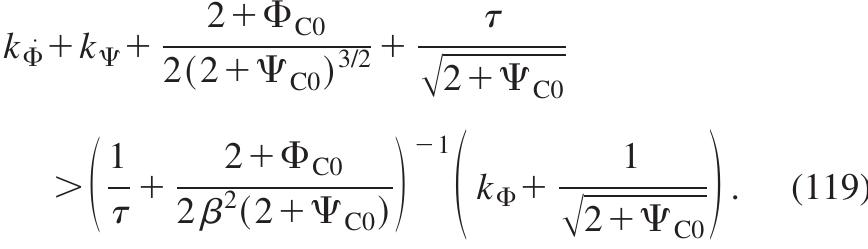
For a cubic characteristic, these conditions have already been re- vealed by Krener [14]. Since these conditions involve not only the shape parameters S$, and S, of the compressor characteristic but also the value of pressure at the peak, 2+W eo, we are of the opinion that controller (23), in which I’ is the bifurcation param- eter, is preferable to the controller (98). where yo is a set point/disturbance parameter and the gains kp, kp, ky, and kq are required to satisfy For right-skew compressors, for which S,;>0 and S,<0, the conditions (99)—(101), in particular, allow controllers of the fol- lowing types:

where &(R)=B?/7VVp,(R). The characteristic polynomial of the Jacobian (117) is Sufficient conditions for stability of the system near the stall in- ception point are readily deduced from (118) and are given in Table 4. A center manifold argument similar to that in Section 6.3 proves stability at the bifurcation point.

8.2 Actuator/Sensor Trade-Off. The time constant 7 ap- pears only in the third condition in Table 4. When cg=0, this condition becomes We point out that in the case of a linear implementation (98) the gains kr, kg», kw, and k@ are required to satisfy condition: (99) and (101), whereas the condition (100) is modified as

Fig. 13 Bifurcation diagrams for the case e=0.9, B=0.71, with the (W,R)-controller. The control gains are cp=3 and cy=1.

Fig. 14 Bifurcation diagrams for the case «e=0.9, G=0.71, with the nonlinear (W,@)-controller. The controls are gain dy=2 and nonlinear function Vy(W).

Fig. 15 Bifurcation diagrams for the case e=0.9, B=1.42, 7=0.44, with the full-state controller. The control gains are Crp=43, Cy=17, and Cy=22.

Table 5 h,(0) for nonlinear implementation Thus, high gain on ® makes a right-skew compressor unstable. Similar but more complicated argument applies to h4(Ro).

Table 7 h,(0) for linear implementation Table 8 h; for linear implementation A discussion similar to that in Section 10.1 shows that the increase of kq results in instability for the right-skew case. Let us now set kp=ky=0 and concentrate on the UTRC controller. Since h,(0) and Ry are independent of kg, for stability we re- quire that h5(0)>0. It is obvious that, for large kg, the sign of h3(0) is determined by the sign of S,S)=—4¥U(1). Thus, the

Since Ro is independent of dg, the sign of h,(0)+h;(0)Ro for large dp is determined by the sign of S,;S,= —4 c(1). This means that, for large do , - For small Ro>O (near the stall inception point), a necessary condition for stability is h,(0)+h;(0)Rj>O. Let us concentrate on The quantities 4,(0) and 4;(0) are given in Tables 5 and 6, re- spectively.

Fig. 16 Closed-loop bifurcation diagrams for e=0.6 with UTRC controller. The control gains are kKp=3 and kg =1,10,100.

The pressure Py can be obtained by substituting the solution (36) into the Eq. (1b), which gives Similarly, the approximate solution of problem (18) is the same as the approximate solution of problem (10), that is, the transfer functions are given by Eqs. (27)—(28). Finally, we consider the approximate solution of problem (19), where flow rate is given at beginning of the line and pressure is given at end of the line. The flow rate solution is given by

Table 1 Some window functions If the trigonometric basis (32) is used with the function

Fig. 1 Imaginary part of the propagation operator ['2(s =ifwT) and its approximations, when friction coefficient « =1/10

The Q model is used when transmission lines are connected together or to fluid volumes (e.g., hydraulic cylinder) by compo- nents of negligible volume such as directional control valves (Fig. 2). Such connectors are modeled as orifices as in Piché & Ellman [18] and Ellman and Piché [19]. The Q-model transfer functions are A 4-mode SIMULINK realization of the Q model is shown in Fig. 3.” Implementation in other simulation environments should be straight forward. Because the models are decoupled, the model has an obvious parallellization. The approximate transfer function (59) are rational polynomials thus inverse Laplace transformation can be calculated giving constant coefficient ordinary differential equations. For ODE-based simulators the following state space realization can be used (with n modes):

Fig. 3 SIMULINK realization of the Q-model with 4 modes 2SIMULINK realization of Q, P, and PQ models of transmission lines are avail- able at ftp.cc.tut.fi/pub/math/piche/fluidpower

Fig.2 A pipe system with Q-pipe models. Pipes are connected by the orifice that simply calculates flow rate through it when pressure drop is known.

Table 2. The physical properties of pipe line system

The PQ model is used when the connections at the ends of the transmission line are of different types. One end can be connected to an orifice and the other directly to a volume. The PO-model transfer functions are The P model is used when transmission lines are connected together to fluid volumes by components of negligible resistance (Fig. 4). Such connectors are modeled as hydraulic volumes (Piché and Ellman [7]). The P-model transfer functions are

Fig. 4 A pipe system with P-pipe models. Pipes are connected to the volume that is modeled by an integrator. More than two pipes may be connected to a single volume.

Pressure in time domain at intermediate points along the transmis- sion line can be calculated using the Ritz approximation (23)

When modeling a network containing several transmission line elements, one should select the number of modes such that the ratio n/L is about the same for each element. This ratio reflects the bandwidth over which the model is supposed to be accurate. Thus, longer transmission lines require more modes to accurately model the same frequency range as shorter lines with fewer modes. Assigning too many modes to short transmission lines is inefficient, since the numerical ODE integrator will need to use small time steps to follow the high frequency modes. This numeri- cal cost would be especially evident with simulators that use BDF methods (such as Gear’s method) as the integrator, because of their inefficiency with oscillatory problems.

Fig. 6 Single pipe example, comparing dissipative (2D vis- cous) and linear friction (1D viscous) models of pressure re- sponse at beginning of line

Fig.5 Single pipe example, pressure response at beginning of line

Fig. 7 Water hammer example pressure response at valve for first cycle of water hammer in high-viscosity oil Table 4 The physical properties of water hammer system in Sl units (Holmboe and Rouleau [20])

Substituting the Ritz approximation into Eq. (70) and simplifying yields the ordinary differential equation system of second order Equations (66a) and (66b) do not include frequency dependent friction effect, since the equations are one-dimensional. Equations (71)—(73) can be modified to include frequency dependent friction effects (2D friction), if we assume that for small flow rate and pressure perturbations the turbulence flow behave the same way as laminar flow. This assumption is related to turbulent mean flow condition in Trikha, [12]. Comparing the Q model (59) and Eq. (72) and (73) we can modify the matrices as follows (2D friction):

Fig. 8 Nonlinear (turbulent) flow example pressure response at beginning of line

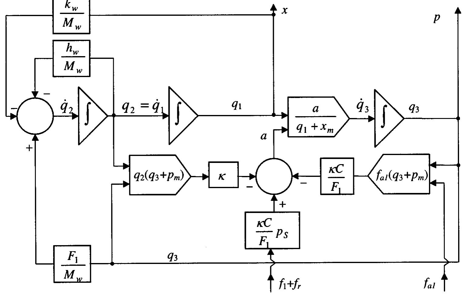
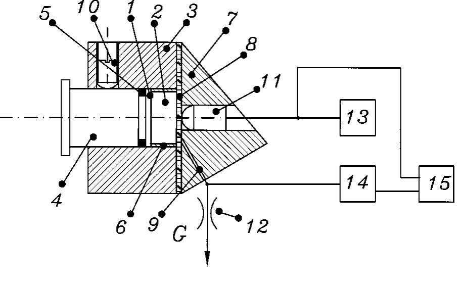
Fig. 1 Diagram of a pneumatic vibration exciter It was experimentally found that in real flow conditions present in a working generator temperature changes can be omitted and Pressure p,, controlled by valves f; and f,,, mainly depends on the quantity of air mass in chamber V,. Changes in the chamber volume caused by piston vibrations have little effect on pressure P1, in the open chamber and air stiffness in such a chamber is, inter alia, dependent on frequency w and is smaller than in the closed chamber [1]. The component of pressure function pj, re- sulting from varying volume of chamber V, is a feedback signal in the generator. When the feedback is compensated, changes in the chamber volume do not cause the air pressure in this chamber to change, thus the air temperature remains unchanged, too. This leads to a conclusion that the air temperature 7, in chamber V, depends mainly (or exclusively after feedback compensation) on air flow processes. _ «2 a el oe In ee

Fig. 2 Physical model of a pneumatic vibration exciter

Assuming the initial conditions g,(0)=0, q2(0)=0, and q3(0) =0, the Eqs. (24) can be solved numerically by one of the The system of Eq. (23) can be written in the state coordinates assuming the notations x=q,, X=q2o, X=q2o, p=q;3; hence

into a variable component chamber /0 and constant component chamber //. There is a cylinder linear in the variable component chamber. The liner consists of four ring segments /2, 13, 14, and 15. Between them are rectangular slots: an inlet 76 and outlet 17. These slots have rectangular cross-sections. Their longer sides with length / are parallel to the cylinder axis. The cylinder liner design allows each segment to turn independently. This, in turn, enables separate width adjustment of both slots b, and b, and the phase angle \, between them (Fig. 5). In Fig. 4 and 5 only one inlet and one outlet slots are shown. In fact, there may be more such slots as described in the earlier work; and they are arranged symmetrically on the cylinder liner wall. If this is the case, the opening functions f; and f,,,; are formed from a number of smaller components. This facilitates achieving the desired character of air flows and enhances the effectiveness of generator operation. The rotor /8, placed in the cylinder liner, is used for harmonic control of the opening function. Its head surfaces have sinusoidal contours with the amplitude A, and nonfractional and identical number of periods on each side. The phase shift angle of the sinusoidal con- tours is zero. The rotor is turned, by a device not shown in the drawing, at a variable (rotating) speed n dependent on the required exciting frequency w. The cylinder liner design with sinusoidal contours of the rotor is shown in Fig. 5. The values of the variable components of the opening functions depend on the angular posi- Fig. 4 Pneumatic vibration generator design for experimental investigation. 7, cylinder; 2,3, covers; 4, two-sided piston; 6,8, inlet holes; 7,9, outlet holes; 10,17, chambers; 12,13, 14,15, ring components of cylinder liner; 76, inlet slot; 77, outlet slot; 78, rotor with sinusoidal contours. Fig.5 A fragment of the extended cylinder liner with inlet and outlet slots, cylindrical rotor surface with sinusoidal contours marked with a broken line; 1,2,3,4, ring components of cylinder liner; 5, inlet slot; 6, outlet slot; 7, rotor with sinusoidal contour

Fig. 3 Variable of a pneumatic exciter state

Fig. 4 Pressure signal versus time for G=0, V,g=30 mm’, F=5Hz; (a) L,=150 wm; V=105 mm’; (b) L,=150 wm V=350 mm; (c) L,=150 wm; V=665 mm; (d) L,=45 wm; V=675 mm*; — experimental data; - - theoretical data

Fig. 2 Geometrical configuration of an OPD with a grid system

Fig. 5 Pressure signal versus time for G=0.5*10-° m%/s Pa, Vag=70mm*: (a) L,=150 um; V=105mm'; F=5 Hz; (b) L,=150 wm; V=200 mm’; F=5 Hz; (c) L,=150 wm; V=350 mm’; F=10 Hz; (d) L,=150 wm; V=665 mm; F=10Hz; — experi- mental data; - - theoretical data

where Ax,At are step sizes in the space and time domain, respec- tively, superscript ‘‘’’ stands for the time step. From Eqs. (4), (7), and (8) we obtain the equation for defining the temperature at the exposed absorbent surface at each time (t+At) step

Fig. 7 Pressure signal versus time for G=0.5*10-° m/s Pa, Vag= 70 mm, L,=150 wm; V=105 mm®: (a) F=10 Hz; (b) F=50 Hz; (c) F=100 Hz; (d) F=200 Hz; — experimental data; - - theoretical data

Fig. 1 Experimental apparatus for the temperature measure- ment (during charging)

Fig. 2 Experimental apparatus for the temperature measure- ment (during discharging)

Fig. 3 Temperature responses during discharge

Fig. 4 Temperature responses during discharge (a) tempera- ture response assuming that the whole heat generated by the expansion of air use transferred to the material

Fig. 6 Experimental results of the steady flow rate measure- ment 5.2. Results and Discussion. Figure 6 shows the pressure curves and the flow rates of the experimental results. The experi- ment was done for four flow rates. Cases 1 to 4 correspond to supply pressures of 542, 444, 346, and 248 kPa, respectively. The

Fig. 7 Experimental apparatus for the unsteady flow rate mea- surement

Fig. 8 Unsteady flow rate measurement with the isothermal chamber (f=5 [Hz])

Fig.9 Unsteady flow rate measurement with isothermal cham- ber (f=40 [Hz])

Fig. 10 Unsteady flow rate measurement with the normal chamber (f= 40 [Hz])

The first term in Eq. (2) is the driving moment from the torque- motor. The last five terms are restoring moments on the armature from the net rotational stiffness, the cantilever feedback spring stiffness (if this spring exists), the damping in the torque-motor, the pressure difference across the nozzle, and the dynamic flow force on the flapper, respectively.

The first two terms in Eq. (6) are the forces from the spool pres- sures and the spool damping, respectively. The next two terms in Eq. (6) are, respectively, the flow reaction force, which depends on the actuator pressures, and the transient flow force, which de- pends on the actuator flow rates. These two terms show the de- pendence of the servovalve on the actuator dynamics given below. The last term in Eq. (6) is the restoring force from the feedback spring, where

Fig. 3 Frequency responses of the servovalve The experimental system consists of a Moog servovalve utiliz- ing a cantilever feedback spring and a 0.9 kg double-ended actua- tor with an effective area of 3.613 e * m? (0.56 in’). The supply pressure is 18.6 MPa (2700 psi). Mobil DTE Light oil is used at an average temperature of 90°F. The actuator and spool are con- nected to linear variable differential transducers (LVDT) with +3 mV noise level. The range of the actuator LVDT is +2.5 V for the total stroke of 0.0254 m (+1 in). While the servo valve physical parameters are not available for model verification, the experi- mental frequency responses for the servovalve and the actuator are measured with a signal analyzer, using a ‘“‘swept sine’’ method that generates fixed-amplitude sine waves of varying fre- quencies. This is then used to validate the model order and struc- ture. It is desired to measure this data near the equilibrium actua- tor position x,,=0. Since the actuator is of type 1 as Eq. (22) indicates, it is difficult to keep the actuator near the equilibrium position in open loop. Therefore, a proportional control loop (gain= 1) is used to create a stabilized plant, as shown in Fig. 2. With different input amplitude levels (15 mV, 30 mV, and 50 mV), the frequency responses of the servovalve and actuator are measured and shown in Figs. 3 and 4, respectively. Using the frequency responses from the three input amplitudes, an averaged frequency response is computed for the servovalve and the actua- tor, and nominal models are fitted through the use of an equation- error method [17].

Fig. 4 Frequency responses of the actuator (dot line: 15 m\ input; dash line: 50 mV input; solid line: model) The nominal model for the averaged actuator frequency re- sponse is found to be

Fig. 5 Comparison of servovalve models (solid line: average of experimental data; dot line: second order model; dash line: third order model; dot-dash line: derived model) not vary much with respect to input amplitude. The averaged ser- vovalve frequency response is shown in Fig. 5 with the best curve fits for the models of Eqs. (24)—(26). The derived servovalve model of Eq. (24) is

Fig. 6 Mixed sensitivity problem as a standard problem The solution of the mixed sensitivity problem provides an ap- proximate solution of the robust performance problem because for any complex numbers ‘‘a’’ and “‘b,”’

Fig. 7 Multiplicative uncertainties of the plant models (dash- dot line: W,;; dot line: W,¢; dash line: W,,)

Fig. 9 Experimental step responses (dash-dot line: using Ks; dot line: using K,; dash line: using K,; solid line: plant) Figure 9 shows the experimental step response using each ro- bust performance controller for a reference amplitude of 30 mV. Better system response is achieved with the more accurate eighth-

Fig.8 Performance weights and experimental sensitivites (dot line: using K, from the second order model; dash line: using K, from the third order model; solid line: using Kg from the derived fifth order model)

Recall that K,=0 for a servovalve with a cantilever feedback spring and K=O for a servovalve with a direct spool feedback spring. ~ The three equations ((Al), (A2), and (A3)) contain three un- knowns: p,)(5)—Ps2(s), O(s), and x,(s). These three unknowns are solved as a function of the input current.

Fig. 1 Adaptive control system block diagram Then the plant equation in (6) becomes

Adaptive Repetitive Control. Since both the reference tra- ectory and disturbance are periodic, S(q~')=1—q~™ may be Note that some coefficients are comparably smaller than others. It is possible to reduce the nominal model to a lower order one. However, to achieve closed-loop stability and better tracking per- formance, we use the 8th-order nominal model so that the size of the unmodeled dynamics « is sufficiently small as suggested by Theorem 1. Indeed, the adaptive control experiment was unstable when using lower order model for the same tracking reference profile.

A cam profile shown in Fig. 3 is used as the tracking reference signal throughout the experiments. To achieve high accuracy, the cam profile consists of 256 points over one spindle rotation, ren- dering 2560 Hz sampling frequency at 600 rpm spindle speed. Throughout the experiment the fluid supply pressure is 20684.4 Kpa (3000 psi) unless otherwise mentioned. Off-line System Identification. Five sets of frequency re- sponse were obtained for the actuator with different actuation am- plitudes by the swept sine method (Fig. 4). The curve fit model shown as solid line in Fig. 4 shows unmodeled dynamics from the real system. The curve fit discrete model considered as the tuned nominal model in Eq. (2) is

Fig. 4 Swept-sine frequency responses at different input magnitudes

Fig. 5 Tracking error and control signal for nonadaptive re- petitive control with perturbed nominal model

Fig. 7 Steady-state tracking error and control signal for adap- tive repetitive control with perturbed nominal model Fig.6 Transient tracking error and control signal for adaptive repetitive control with perturbed nominal model

Fig. 8 Tracking errors of nonadaptive and adaptive repetitive control at 13789.6 Kpa (2000 psi)

Fig. 9 Tracking errors of nonadaptive and adaptive repetitive control at 10342.2 Kpa (1500 psi) The order of the closed-loop characteristic polynomial for the repetitive control system is usually high and has poles close to the unit circle. Thus the closed-loop system becomes unstable with the slight perturbation. All industrial actuators have manufactur- ing variations. If a fixed repetitive controller is applied to several actuators, it may not be stable due to parameter mismatch. An adaptive repetitive controller can handle the parameter mismatch and adapt itself to new controller gains.

Since the right-hand side of the above inequality is nondecreas- ing, we have

(II): r(k)=0 since S(q~')y,e(k)=0. Also since ||¢(k)|| is bounded from (I), we have D(k) €1,5D €1,>D(k)—0. With X=max(A.Ay), (A2) and (A3) imply that The RHS of the above inequality is nondecreasing. Provided that e<X(1—X)/(k,||v|]) we have Further, § has no common factor with B, by assumption, there exist polynomials 7 and A, such that yS+AB,=1. Therefore, xSu+ABu=u and xi+A(A,y—C,d)=u. Therefore u(k) is bounded since the left hand side of the above is bounded. Since || @(n)||Skgl|x(n)|| and D(n) €1,, by the discrete form of the Bellman-Gronwall’s lemma (see Lemma 3), ||x(k)|| is bounded. Therefore # and y are bounded.

Under ideal conditions, where the load torque is zero and sys- tem parameters such as inertia load and supply pressure are con- stant, the required response may be achieved by the proper design of a controller using the pole-placement technique. Hence, con- ventional controllers are designed to such nominal conditions. However, in real systems, load torque disturbances and variations in system parameters, such as inertia load and supply pressure, The transfer functions of the speed response for input command and external load torque are obtained as follows from Fig. 3: Figure 3 shows a block diagram of the system with a conven- tional cascade speed controller. The basic control structure is a double loop, which consists of an inner proportional position- control loop and an outer proportional and integral speed-control loop.

Fig. 3 Block diagram of the conventional control system

Fig. 1 Schematic diagram of VDHM control system

Fig. 4 Block diagram of the proposed control system

Table 1 System parameters Figure 7 is a schematic diagram illustrating the experimental setup. It consists of three parts: a motor system, a load generating system, and a data acquisition and control system. Some of the technical specifications of the experimental setup are as follows: the sampling period is 1 ms, the servovalve rated current is 60 mA, and the rated flow is 30 l/min at a pressure drop of 70 bar. The max. displacement volume of the VDHM is 40 cc/rev, the encoder resolution and the A/D, D/A converters are 1000 pulse/ rev and 12 bits, respectively. Bandwidth of the amplifier for the LVDT is 500 Hz and that of the signal conditioner for the torque sensor is 15 kHz. The signal of the motor speed from the encoder is so noisy that a low-pass filter with a bandwidth of 50 Hz is used. The nominal operating conditions of input speed command, inertia load, and supply pressure are 1000 rpm, 0.04 kgm? (8 times of motor shaft inertia J,), and 150 bar, respectively. Some of the experimental conditions are given as follows:

The transfer function G(s) can be obtained from Fig. 4 as fol lows:

Fig. 8 Comparison of measured and observed torque

Fig. 10 Response for the sinusoidal load torque Fig. 9 Response for the step load torque

Table 2 Overshoot for various 7, and 7, (J=2J,).

Fig. 11 Step response for the input change

Fig. 12 Step response for the change of inertia (dotted line: conventional PI controller, real line: proposed controller)

It is herein noted that the yield stress of the ER fluid employed in this work gradually increases as the temperature increases to about 90°C, and sharply decreases above 90°C, as shown in Fig. 1(b). This is due to that as the temperature increases, the polar- ization effect of the conductive particles becomes more active. This microscopic phenomenon results in the increment of the yield stress. However, it is observed that the field-dependent ER effect significantly degrades above 90°C, since the particles of the employed ER fluid start melting around 90°C. The information on the variation of the ER effect with respect to the temperature is

Fig. 1 Bingham property of the employed ER fluid. (a) Shear stress, (b) yield stress.

Fig. 3 The manufactured cylindrical ER valve. (a) Assembly drawing, (b) photograph.

Fig. 4 Field-dependent step responses of the ER valve

Now, from the above equations, a state-space model for the governing equation of motion of the proposed ER valve bridge- cylinder system can be written as follows:

Fig. 7 A neural network controller incorporating the PID con- troller. (a) Block-diagram, (b) network architecture.

Fig. 9 Set position control responses without cart. (a) Simu- lated, (b) measured. component of the cart is numerically obtained by differentiating the displacement signal. The pump makes a flow of the ER fluid, and thus the piston rod of the cylinder is moved. The temperature of the operating ER fluid is maintained at 55°C during control action by operating the air cooling system. The flow rate of the ER fluid from the pump is chosen by 8 I/min. The displacement of the cart is measured and compared with the desired displacement. In order to minimize the position error, the control electric field

Fig. 8 Experimental configuration for the position control. (a) Schematic diagram, (b) photograph.

Fig. 10 Set position control responses with cart. (a) Simu- lated, (b) measured.

Fig. 11 Square trajectory tracking control responses with cart. (a) Simulated, (b) measured.

Fig. 12 Sinusoidal trajectory tracking control responses with cart. (a) Simulated, (b) measured.

Fig. 14 Measured tracking durability of the control system Fig. 13 Comparison of measured tracking responses with cart. (a) Neural network, (b) PID.

Fig. 1 Cylinder head arrangement of a digital-displacement pump-motor Figure 3 shows a schematic representation of a motoring cycle [4]. To enable a cylinder for motoring the controller closes the low-pressure valve shortly before the piston reaches the top-dead- center (TDC). Once the valve is closed, the cylinder pressure rises to equal to that of the high-pressure manifold by the time it reaches TDC. The high-pressure valve can then be opened and latched. The piston is then propelled by the fluid pressure toward BDC. In a similar fashion to the TDC valve-sequence, the high- pressure valve is closed prior to BDC such that the residual piston stroke can de-pressurize the cylinder and allow the low-pressure

Fig. 2 Change of the enabling sequences of a 10 cylinder pump and its effect on flow as the demand drops to 3/4th of the capacity

Fig. 4 Pump response at 10 percent to 90 percent step rise of flow demand at a constant speed (pressure-control mode) The displacement out of the accumulator S$, can be calculated from the pressure difference between the current and the previous decisions:

Fig. 5 Pump response to 17 percent speed change, while the flow demand remains constant (pressure-control mode)

Fig.6 Pump-motor following a variable demand curve at 1800 rpm (flow-control) Pave=a running average of pressure of last 5 decisions

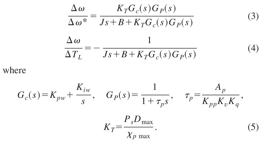
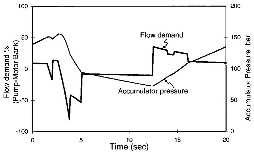
The digital-displacement technology has advanced in the last few years both in terms of compu ter simulation and the building of prototypes. The first prototype of a six-cylinder pump was built in 1990. The single cylinder pump-motor prototype (1994) was followed by a six-cylinder axial pump-motor (1996). Figure 13 shows a photograph of the various components used for a six- cylinder radial pump-motor whic writing. Experimental work has simulations, some of which have Figure 14 shows the experimenta motor, running at 1500 rpm und h is under test at the time of shown good agreement with already been published [3,4]. results of a 6-cylinder pump- er pressure-control mode. The pressure is held constant (about 70 bars) while the pump flow follows an increase from 10 to 90 percent of the capacity in about 30 ms. The experimentally measured response time of the digital- Fig. 9 Power requirement of the pump-motor bank

ry [he second bank also consists of a 10 cylinder machine, which only acts as a pump and which is sized to provide the maximum flow demanded by the load. The cylinder enabling sequence is dictated to follow the flow requirement of the load, converting the shaft output to hydraulic power. Figure 11 shows the output flow from the second bank as well as the flow-demand. Figure 12 shows the power output from the system compared to the load- demand. It also shows the much smaller constant power contribu- tion of the prime-mover.

Fig. 13 Components of a 6-cylinder pump-motor

Fig. 11 Demand and flow from second bank (pump)

Fig. 1 General machine configuration While the valve plate is held in a fixed position, the coupled shaft and cylinder block are driven about the x-axis at a angular speed, w, which will also be considered a constant in the follow- ing analysis. During this motion, each piston periodically passes over the discharge and intake ports on the valve plate. Further- more, because the slippers are held against the inclined plane of the swash plate, the pistons undergo an oscillatory displacement in and out of the cylinder block. As the pistons pass over the intake port, the piston withdraws from the cylinder block and fluid is drawn into the piston bore. As the pistons pass over the discharge port, the piston advances into the cylinder block and fluid is

where A, is the effective pressurized area within a single piston bore of the cylinder block and will be discussed later. Similar to Eq. (1), the forces acting on the cylinder block in the y- and z-directions may be summed and set equal to zero as follows:

where E,, and E, locate the centroid of the valve-plate reaction force, F,,. Summing the moments acting on the cylinder block about the origin of the y- and z-axis and setting them equal to zero yields the following results: Piston-Slipper Assembly Free-Body-Diagram. The forces acting on a single piston-slipper assembly are shown in Fig. 3. These forces result from the pressure within the nth piston bore (A,P,,), the equal and opposite reaction of the cylinder block against the nth piston (—F), and —F7, ), and the net reaction between the nth slipper and the swash plate (F sw, )* Summing the forces acting on the nth piston-slipper assembly in the x-direction and setting them equal to the time rate-of-change of linear mo- mentum for the entire assembly in this direction yields the follow- ing result:

Fig. 3 Piston-slipper assembly free-body-diagram

Fig. 4 Schematic of a piston-bore control volume For a constant speed machine dt=d6/w. Using this result with Eqs. (12), (13), and (14), the pressure rise-rate within a single piston chamber may be written as

Equation (15) is a nonlinear, first-order, differential equation that must be solved numerically. Figure 5 shows a typical numeri- cal result of Eq. (15). Note that both pressure, P, and port area, A,, are plotted in this figure. As shown in Fig. 5, the typical numerical solution to Eq. (15) demonstrates rather uninteresting behavior for the pressure, P. As the piston bore passes over either the intake port or the discharge port of the valve plate, the port area, A, , remains at a maximum constant. Within these regions, the pressure within the nth piston-bore also appears to remain fairly constant (i.e, P=P; or Pz). The two ports on the valve plate are bridged by transition regions where A, goes from a maximum value to a minimum value, slowly grows within the transition slot, and then quickly returns to the original maximum value. As the nth piston-bore passes over the transition regions, the pressure changes almost linearly from one port pressure to the other. Fig. 5 A numerical pressure-profile for the nth piston exhibit- ing essentially no overshoot or undershoot in the transition regions

Fig.6 A numerical pressure-profile for the nth piston exhibit- ing overshoot and undershoot in the transition regions Figure 6 shows another result of this study where the pressure drop between ports has been reduced. Figure 6 represents a run using one sixth of the discharge pressure of Fig. 5. From Fig. 6 it can be seen that a lower pressure drop between ports tends to create significant pressure spikes within the transition regions of the valve plate. The reason for this peculiarity is strictly a result of the volumetric compression and expansion within the chamber. In the first case, the chamber volume decreases at a rate faster than the fluid can squeeze out through the port. If the boundary pres- sure is not sufficiently large compared to the starting pressure, volumetric compression of the fluid will cause the pressure within the piston bore to overshoot the approaching boundary condition.

Fig. 8 A schematic of the pressure-profile on the cylinder block near the valve plate.

Fig. 1 Schematic of speed control system-turbine-hydraulic pump network When air is initially supplied to the governor, the piston is held in its innermost position by a spring. In this position, the air inlet ports are open. The influx of air increases P. until the control valve opens the butterfly valve and allows air to flow past the turbine, thereby accelerating both it and the governor. Accelera-

tion continues until centrifugal force acting on the piston over- comes the preload force of the piston spring, thus allowing the ait inlet ports to be closed. Figure 2 shows the piston in its steady state position. Here, both the air inlet ports and exhaust ports are closed, thereby maintaining a constant P,.. and butterfly valve po- sition. If the governor overshoots its steady state speed, the piston will move outward to open the air exhaust ports to reduce P., and, in turn, move the butterfly valve to restrict air flow to the turbine.

Fig. 6 Model performance curves when the control valve ori- fice is installed but the transient control orifice is not (Design #2) Fig. 5 Model performance curves when both the transient control orifice and the control valve orifice are installed (De- sign #1)

Fig. 3 Following a discontinuous wall: real (solid line) and es- timated (dashed-line) robot trajectory where g is a positive threshold value, P,(k|k) is an estimate of the covariance matrix of the state (used by the EKF) and Xx (k|k—1) is the time update of the EKF. Moreover, [F(k) — G(X(k|k- 1))] will produce incorrelated time series. On the other hand, if the model is wrong, both the aforementioned conditions will fail. Henceforth, by including the test (23) and the correlation test in a higher level controller, it is possible to perform a wall-following task of discontinuous profiles, by alternatively selecting whether to use the environmental model information to get better estimates of the robot position, or to upgrade the model itself. Figure 3

Fig. 1. Inverse Nichols chart showing curvature of M=0 dB and M=—6 dB

Fig. 3 Template illustrated before removal of interior points— 1000 points Fig. 2 Relationship between specification in dB and minimum radius (in nepers or radians) on the log-polar plane

Fig. 4 Template after removal of interior points—220 points

By LaSalle’s theorem [7], the tracking errors e; and e4 converge to zero globally. In addition, if the condition of persistent excita- tion is satisfied, the parameter estimate will converge to its true value.

Table 1 Values of system and controller parameters ‘I: Mechanical constants, II: Hydraulic constants, III: Friction parameters, IV: Controller parameters 1.0344 10’ Pascal is equivalent to 1500 psi.

Fig. 4 1 Hz force tracking. Desired trajectory: ———, actu: trajectory: —.

Fig. 7 Valve tracking error for 1 Hz force tracking Fig. 6 Valve position for 1 Hz force tracking. Desired trajec- tory: ———,, actual trajectory: ——.

Fig. 8 1 Hz pressure tracking result. Desired trajectory: —

Fig. 11 25 Hz pressure tracking result. Desired trajectory: ——-—, actual trajectory: —. Fig. 10 Friction model verification: 1 Hz pressure tracking.

Differentiating J with respect to K (see p. 592 of [15]), we obtain the optimum value of K.

Fig. 2 Comparison of the frequency responses of the thirty mode model of the beam with its two mode model and a two mode model with a correcting zero-frequency term References

Fig. 1 A schematic of the atomic force microscope

where A, and A, are the Hamaker constants for the attractive and repulsive potentials. Such potential indicates long range attractive forces and short range strong repulsive forces acting on the tip. The net energy of the system scaled by the effective mass m of the cantilever is given by H(x,x',Z) with 3 Numerical Analysis

-ig. 3 Phase portrait for the unperturbed system Let us consider the system in Eq. (8), where the parameters have been set as follows [3]:

Fig. 5 Bifurcation diagram of the AFM model When a small perturbation is added (€=0.1) and for small values of I’ such that A/T >(A/T),., the system shows stable

Fig. 4 Trajectories in the phase plane: (a) F=10; (b) [=11; (c) F=16.2; (d) F=20

Fig. 6 Sensitive dependence on initial conditions: position er. ror for i.c. differing by 0.1%

Fig. 7 Power spectral densities of the tip position é, ; (a) F=10; (b) F=11; (c) F=16.2; (d) F=20. To compute the spectra, an FFT algorithm has been used on a window of 4096 data points collected at a sampling rate of 50 rad/s.

Fig. 8 Poincaré map of the AFM model (10,000 points), I =20, 0=0

Fig. 9 Period doubling bifurcation curve in the (I, a) plane: the region of chaotic attractors lies in a subset of the right side of the curve. The dashed line separates the region of validity for the Melnikov theory.

Fig. 10 Poincaré map of the AFM model (10,000 points), | =20, a=0.8, 0=0

References (506)

Newcomb, R. W., 1966, Linear Multiport Synthesis, McGraw-Hill, New York.
Desoer, C. A., and Vidyasagar, M., 1975, Feedback Systems: Input-Output Properties, Academic Press, New York.
͓3͔ Gevarter, W. B., 1970, ''Basic Relations for Control of Flexible Vehicles,'' AIAA J., 8, pp. 666-672.
͓4͔ Hughes, D., and Wen, J. T., 1996, ''Passivity Motivated Controller Design for Flexible Structures,'' AIAA J. Guid. Control Dynam., 19, pp. 726-729.
Lee, F. C., Flashner, H., and Safonov, M. G., 1995, ''Positivity-Based Control System Synthesis Using Alternating LMIs,'' Proceedings of American Control Conference, Seattle, WA, American Automatic Control Council, Evanston, IL, pp. 1469-1473.
͓6͔ Benhabib, R. J., Iwens, R. P., and Jackson, R. L., 1981, ''Stability of Large Space Structure Control Systems Using Positivity Concepts,'' AIAA J. Guid. Control, 4, pp. 487-494.
͓7͔ McLaren, M. D., and Slater, G. L., 1987, ''Robust Multivariable Control of Large Space Structures Using Positivity,'' AIAA J. Guid. Control Dynam., 10, pp. 393-400.
Lozano-Leal, R. and Joshi, S. M., 1988, ''On the Design of Dissipative LQG- Type Controllers,'' Proc. 27th IEEE Decision and Control Conference, Dec., 2, pp. 1645-1646.
͓9͔ Haddad, W. M., Bernstein, D. S., and Wang, Y. W., 1994, ''Dissipative H 2 /H ϱ Controller Synthesis,'' IEEE Trans. Autom. Control., 39, pp. 827- 831.
Damaren, C. J., 1996, ''Gain Scheduled SPR Controllers for Nonlinear Flex- ible Systems,'' ASME J. Dyn. Syst., Meas., Control, 118, pp. 698-703.
͓11͔ Takegaki, M. and Arimoto, S., 1981, ''A New Feedback Method for Dynamic Control of Manipulators,'' ASME J. Dyn. Syst., Meas., Control, 103, pp. 119- 125.
Ortega, R. and Spong, M. W., 1989, ''Adaptive Motion Control of Rigid Robots: A Tutorial,'' Automatica, 25, pp. 877-888.
Damaren, C. J., 1995, ''Passivity Analysis for Flexible Multilink Space Ma- nipulators,'' AIAA J. Guid. Control Dynam., 18, pp. 272-279.
Damaren, C. J., 1998, ''Modal Properties and Control System Design for Two-Link Flexible Manipulators,'' Int. J. Robot. Res., 17, pp. 667-678.
References ͓1͔ Tyan, F., and Bernstein, D. S., 1994, ''Antiwindup Compensator Synthesis for Systems with Saturating Actuators,'' Proceedings of the 33rd Conference on Decision and Control, 1, pp. 150-155.
͓2͔ Nicolao, D. G., Scattolini, R., and Sala, G., 1996, ''An Adaptive Predictive Regulator with Input Saturations,'' Automatica, 32, pp. 597-601.
͓3͔ Feng, T., 1995, ''Robust Stability and Performance Analysis for Systems with Saturation and Parameter Uncertainty,'' Ph.D. thesis, University of Michigan, Ann Arbor.
Teel, A. R., and Kapoor, N., 1997, ''Uniting Local and Global Controllers for the Caltech Deducted Fan,'' Am. Control Conference, 3, pp. 1539-1543.
Peng, Y., Vrancic, D., and Hanus, R., 1996, ''Anti-Windup, Bumpless, and Conditioned Techniques for PID Controllers,'' IEEE Control Syst. Mag., 16, pp. 48-57.
͓6͔ Khayyat, A. A., Heinrichs, B., and Sepehri, N., 1996, ''A Modified Rate- Varying Integral Controller,'' Mechatronics, 6, pp. 367-376.
͓7͔ Yang, S., and Leu, M. C., 1989, ''Stability and Performance of a Control System with an Intelligent Limiter,'' Proceedings of the 1989 American Con- trol Conference, pp. 1699-1705.
͓8͔ Yang, S., and Leu, M. C., 1993, ''Anti-Windup Control of Second-Order Plants with Saturation nonlinearity,'' ASME J. Dyn. Syst., Meas., Control, 115, pp. 715-720.
͓9͔ Fertik, H. A., and Ross, S. W., 1967, ''Direct Digital Control Algorithm with Anti-Windup Feature,'' ISA Trans., 6, pp. 317-328.
Gilbert, E. G., and Kolmanovsky, I., 1995, ''Discrete-Time Reference Gov- erners for Systems with State and Control Constraints and Disturbance In- puts,'' Proceedings of the 34th Conference on Decision and Control, pp. 1189-1194.
Wredenhagen, G. F., and Belanger, P. R., 1994, ''Piecewice-Linear LQ Con- trol for Systems with Input Constraints,'' Automatica, 30, pp. 403-416.
͓12͔ Larsson, P. T., ''Controller Design for Linear Systems Subject to Actuator Saturation,'' Ph.D. thesis, University of Michigan.
Gutman, P.-O., and Hagander, P., 1985, ''A New Design of Constrained Con- trollers for linear systems,'' IEEE Trans. Autom. Control., 30, Jan, pp. 22-33.
͓14͔ Bernstein, D. S., 1995, ''Optimal Nonlinear, but Continuous, Feedback Con- trol of Systems with saturating actuators,'' Int. J. Control, 62, pp. 1209-1216.
͓15͔ Kazunoba, Y., and Kawabe, H., 1992, ''A Design of Saturating Control with a Guaranteed Cost and its Application to the Crane Control System,'' IEEE Trans. Autom. Control., 37, pp. 121-127.
͓16͔ Larsson, P. T., 1999, Controller Design for Linear Systems Subject to Actuator Constraints, Ph.D. thesis, University of Michigan.
Larsson, P. T., and Ulsoy, A. G., 1998, ''Scaling the Speed of Response Using LQR Design,'' Proceedings of the Conference on Decision and Control, Vol. 1, pp. 1171-1176.
͓18͔ Goldfarb, M., and Sirithanapipat, T., 1997, ''Performance-Based Selection of PD Control Gains for Servo Systems with Actuator Saturation,'' Proc. ASME J. Dyn. Syst., Meas., Control Division, 61, pp. 497-501.
͓19͔ Kamenetskiy, V. A., 1996, ''The Choice of a Lyapunov Function for Close Approximation of the set of Linear Stabilization,'' Proceedings of the 35th Conference on Decision and Control, Vol. 1, pp. 1059-1060.
͓20͔ Tarbouriech, S., and Burgat, C., 1992, ''Class of Globally Stable Saturated State Feedback Regulators,'' Int. J. Systems Sci., 23, pp. 1965-1976.
͓21͔ Burgat, C., and Tarbouriech, S., 1992, ''Global Stability of Linear Systems with Saturated Controls,'' Int. J. Syst. Sci., 23, pp. 37-56.
Gyugyi, P. J., and Franklin, G., 1993, ''Multivariable Integral Control with Input Constraints,'' Proceedings of the 32nd Conference on Decision and Control, 3, pp. 2505-2510.
͓23͔ Phelan, R. M., 1977, Automatic Control Systems, Cornell University Press, Ltd.
Hsu, J. C., and Meyer, A. U., 1968, Modern Control Principles and Applica- tions, McGraw-Hill.
References ͓1͔ Meieran, H. B., and Gelhaus, F. E., 1986, ''Mobile Robots Designed for Haz- ardous Environments,'' Robots and Engineering, 8, pp. 10-16.
͓2͔ Wilcox, B., et al., 1992, ''Robotic Vehicles for Planetary Exploration,'' IEEE International Conference on Robotics and Automation, pp. 175-80.
͓3͔ Woodbury, R., 1990, ''Exploring the Ocean's Frontiers Robots and Miniature Submarines Take Oil Drillers to New Depths.'' Time, 17.
Schneider, S. A., and Cannon, R. H., Jr., 1992, ''Object Manipulation Control for Cooperative Manipulation: Theory and Experimental Results,'' IEEE Trans. Rob. Autom., 8, No. 3, pp. 383-394.
͓5͔ Luk, B., Collie, A., and Bingsley, J., 1991, ''Robug II: An Intelligent Wall Climbing Robot,'' Proceedings of the IEEE International Conference on Ro- botics and Automation, Sacramento, CA, Vol. 3, pp. 2342-2347.
͓6͔ Gorinevsky, D., and Schneider, A., 1990, ''Force Control in Locomotion of Legged Vehicles over Rigid and Soft Surfaces,'' Int. J. Rob. Res., 9, No. 2, pp. 4-23.
Yoneda, K., Iiyama, H., Hirose, and Shigeo, S., 1994, ''Sky Hook Suspension Control of a Quadruped Walking Vehicle,'' Proceedings of the IEEE Interna- tional Conference on Robotics and Automation, San Diego, CA, Vol. 2, pp. 999-1004.
Fujimoto, Y. and Kawamura, A., 1996, ''Proposal of Biped Walking Control Based on Robust Hybrid Position/Force Control,'' Proceedings of the IEEE International Conference on Robotics and Automation, Minneapolis, MN, Vol. 4, pp. 2724-2730.
Celaya, E. and Porta, J., 1996, ''Control of a Six-Legged Robot Walking on Abrupt Terrain,'' Proceedings of the IEEE International Conference on Ro- botics and Automation, Minneapolis, MN, Vol. 4, pp. 2731-2736.
Sunada, C., Argaez, D., Dubowsky, S., and Mavroidis, C., 1994, ''A Coordi- nated Jacobian Transpose Control for Mobile Multilimbed Robotic Systems,'' References ͓1͔ Kanellakopoulos, I., Kokotovic ´, P. V., and Morse, A. S., 1991, ''Systematic Design of Adaptive Controllers for Feedback Linearizable Systems,'' IEEE Trans. Autom. Control., 36, pp. 1241-1253.
͓2͔ Krstic ´, M., Kanellakopoulos, I., and Kokotovic ´, P. V., 1992, ''Adaptive Non- linear Control Without Over-Parameterization,'' Systems Control Lett., 19, pp. 177-185.
Krstic ´, M., and Kokotovic ´, P. V., 1995, ''Adaptive Nonlinear Design with Controller-Identifier Separation and Swapping,'' IEEE Trans. Autom. Con- trol., 40, pp. 426-440.
͓4͔ Nam, K., and Arapostathis, A., 1988, ''A Model Reference Adaptive Control Scheme for Pure-Feedback Non Linear Systems,'' IEEE Trans. Autom. Con- trol., 33, pp. 803-811.
͓5͔ Seto, D., Annaswamy, A. M., and Baillieul, J., 1994, ''Adaptive Control of a Class of Nonlinear Systems with a Triangular Structure,'' IEEE Trans. Autom. Control., 39, pp. 1411-1428.
͓6͔ Utkin, V. I., 1992, Sliding Modes In Control And Optimization, Springer- Verlag, Berlin.
Zinober, A. S. I. ed., 1994, Variable Structure and Lyapunov Control, Springer-Verlag, London.
͓8͔ Bartolini, G., and Ferrara, A., 1994, ''Model-Following VSC Using an Input- Output Approach,'' Variable Structure and Lyapunov Control, A.S.I. Zinober, ed., Springer-Verlag, London, pp. 289-312.
͓9͔ Narendra, K. S., and Boskovic, J. D., 1989, ''A Combined Direct, Indirect and Variable Structure Method for Robust Adaptive Control,'' IEEE Trans. Au- tom. Control., 37, pp. 262-268.
͓10͔ Bartolini, G. Ferrara, A., Giacomini, L., and Usai, E., 1996, ''A Combined Backstepping/Second Order Sliding Mode Approach to Control a Class of Nonlinear Systems,'' Proc. IEEE International Workshop on Variable Struc- ture Systems, Tokyo, Japan, pp. 205-210.
͓11͔ Sira-Ramirez, H., 1992, ''On the Sliding Mode Control of Nonlinear Sys- tems,'' Systems Control Lett., 19, pp. 303-312.
͓12͔ Zinober, A. S. I., and Rios-Bolivar, E. M., 1994, ''Sliding Mode Control for Uncertain Linearizable Nonlinear Systems: A Backstepping Approach,'' Proc. IEEE Workshop on Robust Control via Variable Structure and Lyapunov Techniques, Benevento, Italy, pp. 78-85.
͓13͔ Bartolini, G., Ferrara, A., and Usai, E., 1997, ''Applications of a Suboptimal Discontinuous Control Algorithm for Uncertain Second Order Systems,'' Int. J. Robust Nonlin. Control, 7, pp. 299-320.
͓14͔ Levant, A., 1993, ''Sliding Order and Sliding Accuracy in Sliding Mode Con- trol,'' Int. J. Control, 58, pp. 1247-1263.
͓15͔ Spong, M. W., and Vidyasagar, M., 1989, Robot Dynamics and Control, Wiley, New York.
͓16͔ Marino, R., and Nicosia, S., 1985, ''Singular Perturbation Techniques in the Adaptive Controls of Elastic Robots,'' Proc. 1st IFAC Symp. on Robot Con- trol, Barcelona, pp. 95-100.
͓17͔ Spong, M. W., 1987, ''Modeling and Control of Elastic Joint Robots,'' ASME J. Dyn. Syst., Meas., Control, 109, pp. 310-319.
͓18͔ Chang, Y., and Daniel, R. W., 1992, ''On the Adaptive Control of Flexible Joint Robots,'' Automatica, 28, pp. 969-974.
͓19͔ Ge, S. S., 1996, ''Adaptive Controller Design for Flexible Joint Manipula- tors,'' Automatica, 32, pp. 273-278.
͓20͔ Spong, M. W., 1989, ''Adaptive Control of Flexible Joint Robots,'' Systems Control Lett., 13, pp. 15-21.
͓21͔ Spong, M. W., 1995, ''Adaptive Control of Flexible Joint Manipulators: Com- ments on Two Papers,'' Automatica, 31, pp. 585-590.
͓22͔ Su, R., and Hunt, L. R., 1986, ''A Canonical Expansion for Nonlinear Sys- tems,'' IEEE Trans. Autom. Control., 31, pp. 670-673.
Krstic ´, M., Kanellakopoulos, I., and Kokotovic ´, P. V., 1995, Nonlinear and Adaptive Control Design, Wiley, New York.
Krstic ´, M., and Kokotovic ´, P. V., 1994, ''Observer-Based Schemes for Adap- tive Nonlinear State-Feedback Control,'' Int. J. Control, 59, No. 6, pp. 1373- 1381.
Jankovic, M., 1997, ''Adaptive Nonlinear Output Feedback Tracking with a Partial High-Gain Observer and Backstepping,'' IEEE Trans. Autom. Control., 42, No. 1, pp. 106-113.
͓26͔ Bartolini, G., Ferrara, A., and Usai, E., 1997, ''Output Tracking Control of Uncertain Nonlinear Second-Order Systems,'' Automatica, 33, No. 12, pp. 2203-2212.
Li, Z., and Krstic ´, M., 1997, ''Maximizing Regions of Attraction Via Back- stepping and CLFs with Singularities,'' Systems Control Lett., 30, pp. 195- 207. References ͓1͔ Arimoto, S., Kawamura, S., and Miyazaki, F., 1984, ''Bettering Operation of Robots by Learning,'' J. Robotic Systems, 1, No. 2, pp. 123-140.
͓2͔ Kwong, W. A., and Passino, K. M., 1995, ''Dynamically Focused Fuzzy Learning Control,'' Proc. American Control Conf., pp. 3755-3759.
͓3͔ Teshnehlab, M., and Watanabe, K., 1995, ''Flexible Structural Learning Con- trol of a Robotic Manipulator Using Artificial Neural Networks,'' JSME Int. J., Series C, 38, No. 3, pp. 510-521.
͓4͔ Yang, B. H., and Asada, H., 1995, ''Progressive Learning for Robotic Assem- bly: Learning Impedance with an Excitation Scheduling Method,'' Proc. IEEE Int. Conf. on Robotics and Automation, pp. 2538-2544.
͓5͔ Horowitz, R., 1993, ''Learning Control of Robot Manipulators,'' ASME J. Dyn. Syst., Meas., Control, 115, No. 2͑B͒, pp. 402-411.
͓6͔ Messner, W., Horowitz, R., Kao, W. W., and Boals, M., 1991, ''A New Adap- tive Learning Rule,'' IEEE Trans. Autom. Control., 36, No. 2, pp. 188-197.
͓7͔ Guglielmo, K., and Sadegh, N., 1996, ''Theory and Implementation of a Re- petitive Robot Controller with Cartesian Trajectory Description,'' ASME J. Dyn. Syst., Meas., Control, 118, No. 1, pp. 15-21.
͓8͔ Guvenc, L., 1996, ''Stability and Performance Robustness Analysis of Repeti- tive Control Systems Using Structured Singular Values,'' ASME J. Dyn. Syst., Meas., Control, 118, No. 3, pp. 593-597.
͓9͔ Emelyanov, S. V., 1967, Variable Structure Control Systems, Nauka, Moscow ͑in Russian͒.
Slotine, J.-J. E., and Li, W., 1991, Applied Nonlinear Control, Prentice-Hall, Englewood Cliffs, N.J. ͓11͔ Gao, W., and Hung, J. C., 1993, ''Variable Structure Control of Nonlinear System: A New Approach,'' IEEE Trans. Ind. Electron., 40, No. 1, pp. 45-56.
͓12͔ Strang, G., 1980, Linear Algebra and Its Applications, 2nd ed., Academic, Press.
Burton, J. A., and Zinober, A. S. I., 1986, ''Continous Approximation of Variable Structure Control,'' Int. J. Syst. Sci., 17, No. 6, pp. 876-885.
͓14͔ NSK Corporation, 1989, Megatorque Motor System: User's Manual, Tokyo, Japan.
Sadegh, N., Horowitz, R., and Tomizuka, M., 1990, ''A Unified Approach to Design of Adaptive and Repetitive Controllers for Robotic Manipulator,'' ASME J. Dyn. Syst., Meas., Control, 112, No. 4, pp. 618-629.
Õ Vol. 122, MARCH 2000 Transactions of the ASME References ͓1͔ Falb, P. L., and Wolovich, W. A., 1967, ''Decoupling in the Design and Synthesis of Multivariable Control Systems,'' IEEE Trans. Autom. Control, AC-12, pp. 651-669.
͓2͔ Porter, W. A., 1969, ''Decoupling of and Inverses for Time-Varying Linear Systems,'' IEEE Trans. Autom. Control, AC-14, pp. 378-380.
͓3͔ Porter, W. A., 1970, ''Diagonalization and Inverses for Nonlinear Systems,'' Int. J. Control, 10, pp. 252-264.
͓4͔ Ha, I. J., and Gilbert, E. G., 1986, ''A Complete Characterization of Decou- pling Control Laws for a General Class of Nonlinear Systems,'' IEEE Trans. Autom. Control, AC-31, pp. 823-830.
͓5͔ Xia, X., 1993, ''Parametrization of Decoupling Control Laws for Affine Non- linear Systems,'' IEEE Trans. Autom. Control, AC-38, pp. 916-928.
͓6͔ Isidori, A., 1996, Nonlinear Control Systems: An Introduction, 3rd Ed., Springer-Verlag, Berlin.
Tsirikos, A. S., 1996, ''Contribution to the Development of New Techniques for the Analysis and Design of Linear and Nonlinear Systems,'' Ph.D. thesis, National Technical University of Athens, Department of Electrical and Com- puter Engineering, Athens.
Morgan, B. S., 1964, ''The Synthesis of Linear Multivariable Systems by State-Variable Feedback,'' IEEE Trans. Autom. Control, AC-9, pp. 405-411.
͓9͔ Suda, N., and Umahashi, K., 1984, ''Decoupling of Nonsquare Systems: A Necessary and Sufficient Condition in Terms of Infinite Zeros,'' Proc. 9th IFAC World Congress, Budapest, 1, pp. 88-93.
͓10͔ Descusse, J., Lafay, J. F., and Malabre, M., 1986, ''A Survey on Morgan's Problem,'' Proc. 25th IEEE Conf. Decision Contr. (CDC), 2, pp. 1289-1294, Athens, Greece.
Descusse, J., Lafay, J. F., and Malabre, M., 1988, ''Solution to Morgan's Problem,'' IEEE Trans. Autom. Control, AC-33, pp. 732-739.
͓12͔ Commault, C., Descusse, J., Dion, J. M., Lafay, J. F., and Malabre, M., 1986, ''New decoupling invariants: The essential orders,'' Int. J. Control, 44, pp. 689-700.
Herrera, H. A. N., and Lafay, J. F., 1993, ''New Results about Morgan's Problem,'' IEEE Trans. Autom. Control, AC-38, pp. 1834-1838.
͓14͔ Glumineau, A., and Moog, C. H., 1992, ''Nonlinear Morgan's Problem: Case of (pϩ1) Inputs and p Outputs,'' IEEE Trans. Autom. Control, AC-37, pp. 1067-1072.
Kamiyama, S., and Furuta, K., 1976, ''Decoupling by Restricted State Feed- back,'' IEEE Trans. Autom. Control, AC-21, pp. 413-415.
͓16͔ Descusse, J., Lafay, J. F., and Kucera, V., 1984, ''Decoupling by Restricted State Feedback: The General Case,'' IEEE Trans. Autom. Control, AC-29, pp. 79-81.
Arvanitis, K. G., 1997, ''Simultaneous Uniform Disturbance Localization and Decoupling of Nonsquare Linear Time-Dependent Analytic Systems via Re- stricted State Feedback,'' IMA J. Math. Control Inf., 14, pp. 371-383.
͓18͔ Arvanitis, K. G., 1998, ''Uniform Decoupling of Nonsquare Linear Time- Varying Analytic Systems via Restricted Static State Feedback,'' J. Franklin Inst., 335B, pp. 359-373.
͓19͔ Tarn, T. J., and Zhan, W., 1991, ''Input-Output Decoupling and Linearization via restricted Static State Feedback,'' Proc. 11th IFAC World Congress, Tal- lin, Estonia, 3, pp. 287-292.
͓20͔ Wonham, W. M., 1979, Linear Multivariable Control: A Geometric Approach, Springer-Verlag, New York.
͓21͔ Isidori, A., Krener, A. J., Gori-Giorgi, C., and Monaco, S., 1981, ''Nonlinear Decoupling via Feedback: A Differential Geometric Approach,'' IEEE Trans. Autom. Control, AC-26, pp. 331-345.
͓22͔ Hirschorn, R. M., 1981, ''͑A, B͒-Invariant Distributions and Disturbance De- coupling of Nonlinear Systems,'' SIAM J. Control Optim., 19, pp. 1-19.
͓23͔ Nijmeijer, H., and Van der Schaft, A., 1983, ''The Disturbance Decoupling Problem for Nonlinear Control Systems,'' IEEE Trans. Autom. Control, AC- 28, pp. 331-345.
͓24͔ Krener, A. J., 1985, ''͑Adf, g͒, ͑adf, g͒ and Locally ͑adf, g͒ Invariant and Controllability Distributions,'' SIAM J. Control Optim., 23, pp. 523-549.
͓25͔ Huijberts, H., 1992, ''A Nonregular Solution to the Nonlinear Dynamic Dis- turbance Decoupling Problem with an Application to a Complete Solution of the Nonlinear Model Matching Problem,'' SIAM J. Control Optim., 30, pp. 350-366.
͓26͔ Arvanitis, K. G., 1994, ''Uniform Disturbance Localization with Simultaneous Uniform Decoupling for Linear Time-Varying Analytic Systems,'' Int. J. Syst. Sci., 25, pp. 1679-1694.
͓27͔ Narikiyo, V., and Izumi, T., 1991, ''On model feedback control for robot manipulators,'' ASME J. Dyn. Syst., Meas., Control, 113, pp. 371-378.
͓28͔ Wie, B., Byun, K. W., and Warren, V. W., 1989, ''New approach to attitude/ momentum control for the space station,'' AIAA J. Guidance, Contr. Dyn., 12, pp. 714-722.
References ͓1͔ Book, W. J., 1993, ''Controlled Motion in an Elastic World,'' ASME J. Dyn. Syst., Meas., Control, 115, No. 2, June, pp. 252-261.
͓2͔ Junkins, J. L., and Kim, Y. 1993, Introduction to Dynamics and Control of Flexible Structures.
Singer, N., and Seering, W., 1990, ''Preshaping Command Inputs to Reduce System Vibration,'' ASME J. Dyn. Syst., Meas., Control, 112, No. 1, Mar., pp. 76-82.
Singh, T., and Vadali, S. R., 1994, ''Robust Time-Optimal Control: A Fre- quency Domain Approach,'' AIAA J. Guid., Contr., Dyn., 17, No. 2, Mar.- Apr., pp. 346-353.
͓5͔ Singhose, W., Seering, W., and Singer, N., 1994, ''Residual Vibration Reduc- tion Using Vector Diagrams to Generate Shaped Inputs,'' ASME J. Mech. Des., 116, No. 2, June, pp. 654-659.
͓6͔ Wie, B., Sinha, R., and Liu, Q., 1993, ''Robust Time-Optimal Control of Uncertain Structural Dynamic Systems,'' AIAA J. Guid., Contr., Dyn., 16, No. 5, Sept.-Oct., pp. 980-983.
͓7͔ Smith, O. J. M., 1957, ''Posicast Control of Damped Oscillatory Systems,'' Proc. of the IRE, Sept., pp. 1249-1255.
͓8͔ Singhose, W., Seering, W., and Singer, N., 1996, ''Input Shaping for Vibration Reduction With Specified Insensitivity to Modeling Errors,'' Proc. Japan-USA Symposium on Flexible Automation, Boston, MA.
Magee, D. P., 1996, ''Optimal Arbitrary Time-Delay Filtering to Minimize Vibration in Elastic Manipulator Systems,'' PhD thesis, Georgia Institute of Technology.
de Roover, D., and Sperling, F. B., 1997, ''Point-to-Point Control of a High Accuracy Positioning Mechanism,'' Proc. American Control Conf., Albuquer- que, NM, June, pp. 1350-1354.
͓11͔ Rappole, B. W., Singer, N. C., and Seering, W. P., 1994, ''Multiple-Mode Impulse Shaping Sequences for Reducing Residual Vibrations,'' 23rd ASME Biennial Mechanisms Conf., Minneapolis, MN, DE-71, pp. 11-16.
͓12͔ Singhose, W., Seering, W., and Singer, N., 1995, ''The Effect of Input Shap- ing on Coordinate Measuring Machine Repeatability,'' Proc. IFToMM World Congress on the Theory of Machines and Mechanisms, Milan, Italy, 4, pp. 2930-2934.
Tuttle, T. D., and Seering, W. P., 1997, ''Experimental Verification of Vibra- tion Reduction,'' AIAA J. Guid., Contr., Dyn., 20, No. 4, July-Aug., pp. 658-664.
Singer, N. C., Singhose, W. E., and Kriikku, E., 1997, ''An Input Shaping Controller Enabling Cranes to Move Without Sway,'' Proc. ANS Topical Meeting on Robotics and Remote Systems, Augusta, GA.
Jansen, J. F., 1992, ''Control and Analysis of a Single-Link Flexible Beam with Experimental Verification,'' ORNL/TM-12198, Oak Ridge National Laboratory.
Magee, D. P., and Book, W., 1995, ''Filtering Micro-Manipulator Wrist Com- mands to Prevent Flexible Base Motion,'' Proc. American Control Conf., Se- attle, WA, June, pp. 924-928.
͓17͔ Feddema, J., Dohrmann, C., Parker, G., Robinett, R., Romero, V., and Schmitt, D., 1997, ''Control for Slosh-Free Motion of an Open Container,'' IEEE Con- trol Systems Magazine, 17, No. 1, Feb., pp. 29-36.
͓18͔ Pao, L. Y., 1997, ''An Analysis of the Frequency, Damping, and Total Insen- sitivities of Input Shaping Designs,'' AIAA J. Guid., Contr., Dyn., 20, No. 5, Sept.-Oct., pp. 909-915.
͓19͔ Kirkpatrick, S., Gellet, C., and Vecchi, M., 1983, ''Optimization by Simulated Annealing,'' Science, pp. 671-680.
van Laarhoven, P. J. M., and Aarts, E. H. L., 1987, Simulated Annealing: Theory and Applications, Reidel Publishing Company.
Pao, L. Y., and Lau, M. A., 1999, ''Expected Residual Vibration of Traditional and Hybrid Input Shaping Designs,'' AIAA J. Guid., Contr., Dyn., 22, No. 1, Jan.-Feb., pp. 162-165.
͓22͔ Bhat, S. P., and Miu, D. K., 1991, ''Solutions to Point-to-Point Control Prob- lems Using Laplace Transform Technique,'' ASME J. Dyn. Syst., Meas., Con- trol, 113, No. 3, Sept., pp. 425-431.
͓23͔ Pao, L. Y., and Singhose, W. E., 1995, ''On the Equivalence of Minimum Time Input Shaping with Traditional Time-Optimal Control,'' Proc. IEEE Conf. Control Applications, Albany, NY, Sept., pp. 1120-1125.
͓24͔ Tuttle, T. D., and Seering, W. P., 1994, ''A Zero-placement Technique for Designing Shaped Inputs to Suppress Multiple-mode Vibration,'' Proc. Ameri- can Control Conf., Baltimore, MD, June, pp. 2533-2537.
͓25͔ Pao, L. Y., Chang, T. N., and Hou, E., 1997, ''Input Shaper Designs for Minimizing the Expected Level of Residual Vibration in Flexible Structures,'' Proc. American Control Conf., Albuquerque, NM, June, pp. 3542-3546.
References ͓1͔ Thomas, C. L., 1995, Introduction to Rapid Prototyping, Univ. of Utah, Salt Lake City, UT.
Hartwig, G., 1997, ''Rapid 3D Modelers,'' Design Engineering, Mar., pp. 37-44.
Prinz, F. B., et al., 1995, ''Processing, Thermal and Mechanical Issues in Microcasting Shape Deposition Manufacturing,'' Proc. of the SFF Symposium, Austin, TX, pp. 118-129.
͓4͔ Doumanidis, C. C., 1994, ''Modeling and Control of Timeshared and Scanned Torch Welding,'' ASME J. Dyn. Syst., Meas., Control, 116, pp. 387-395.
͓5͔ Kutay, A., and Weiss, L. E., 1992, ''A Case Study of a Thermal Spraying Robot,'' Robotics Computer-Integrated Manufacturing, 9, No. 4, pp. 12-19.
͓6͔ Doumanidis, C., 1992, ''Hybrid Modeling for Control of Weld Pool Dimen- sions,'' ASME 1992 Japan-USA Symposium on Flexible Automation, San Francisco, CA, July, pp. 317-323.
͓7͔ Goldak, J., 1989, ''Modeling Thermal Stresses and Distortions in Welds,'' Trends in Welding Research, ASM Intl., Gatlinburg, TN, May, pp. 71-81.
͓8͔ Thorn, K., Feenstra, M., Young, J. C., Lawson, W. H. S., and Kerr, H. W., 1982, ''The Interaction of Process Variables,'' Metal Construction 14/3, Mar., pp. 128-133.
Vroman, A. R., and Brandt, H., 1978, ''Feedback Control of GTA Welding Using Puddle Width Measurement,'' Weld. J. ͑Miami͒, 57, Sept, pp. 742-746.
͓10͔ Song, J. B., and Hardt, D. E., 1991, ''Multivariable Adaptive Control of Bead Geometry in GMA Welding,'' ASME Symposium on Welding, 1991, pp. 41- 48.
Hale, M. B., and Hardt, D. E., 1992, ''Multi-Output Process Dynamics of GMAW: Limits to Control,'' Welding Science and Technology, ASM, Gatlin- burg, TN, pp. 1015-1020.
͓12͔ Dornfeld, D. A., Tomizuka, M., and Langari, G., 1982, ''Modeling and Adap- tive Control of Arc Welding Processes,'' Measurement & Control for Batch Manuf., Nov., pp. 53-64
Zhang, Y. M., and Kovacevic, R., 1995, ''Modeling and Real-Time Identifi- cation of Weld Pool Characteristics for Intelligent Controll,'' Proc. 1st World Congress on Intelligent Manufacturing Processes and Systems, 2, pp. 1014- 1023.
Tzafestas, S. G. editor, 1982, Distributed Parameter Control Systems, Perga- mon Press, Oxford, UK.
Ray, W. H., and Lainiotis, D. G., 1978, DPS-Identification, Estimation and Control, Dekker, New York, NY, 1978.
Curtain, R. F., and Pritchard, A. J., 1978, ''Infinite Dimensional Linear Sys- tems Theory,'' Springer-Systems, SIAM J. Control, 10, pp. 329-333.
͓17͔ Delfour, and Mitter, 1972, ''Controllability and Observability for Infinite- Dimensional Systems,'' SIAM J. Control, 10, pp. 329-333.
͓18͔ Alifanov, O. M., 1994, Inverse Heat Transfer Problems, Springer-Verlag, Berlin.
Murio, D. A., 1993, The Mollification Method and the Numerical Solution of III-Posed Problems, Wiley, New York, NY.
͓20͔ Beck, J. V., 1985, Inverse Heat Conduction: Ill-Posed Problems, Wiley, New York, NY.
Marquis, B. P., and Doumanidis, C. C., 1993, ''Distributed-Parameter Simu- lation of the Scan Welding Process,'' IASTED Conf. on Modeling & Simula- tion, Pittsburgh, PA, pp. 146-149.
͓22͔ Batchelor, G. K., 1967, Introduction to Fluid Dynamics, Cambridge Press, London, U.K.
Carslaw, H. S., and Jaeger, J. C., 1959, Conduction of Heat in Solids, 2nd Edition, Oxford Press, London, U.K.
Astrom, K. J., and Wittenmark, B., 1995, Computer-Controlled Systems, 3rd Edition, Prentice-Hall, Englewood Cliffs, NJ.
References ͓1͔ Ibrahim, R. A., 1992, ''Friction-Induced Vibration, Chatter, Squeal, and Chaos: Part I-Mechanics of Friction and Part II-Dynamics and Modeling,'' DE-Vol. 49, Friction-Induced Vibration, Chatter, Squeal, and Chaos, ASME 1992.
Moore, D. F., 1972, ''On the Decrease in Contact Area for Spheres and Cyl- inders Rolling on a Viscoelastic Plane,'' Wear, 21, pp. 179-194.
͓3͔ Moore, D. F., and Geyer, W., 1974, ''A Review of Hysteresis Theories for Elastomers,'' Wear, 30, pp. 1-34.
͓4͔ Barquins, M., and Roberts, A. D., 1986, ''Rubber Friction Variation with Rate and Temperature: Some New Observations,'' J. Phys. D: Appl. Phys., 19, pp. 547-563.
Briscoe, B. J., 1992, ''Friction of Organic Polymers,'' Fundamentals of Fric- tion: Macroscopic and Microscopic Processes, I. L. Singer and H. M. Pollock, eds., Kluwer Academic Publishers, Boston.
Schallamach, A., 1971, ''How Does Rubber Slide,'' Wear, 17, pp. 301-312.
͓7͔ Barquins, M., 1985, ''Sliding Friction of Rubber and Schallamach Waves-A Review,'' Mater. Sci. Eng., 73, pp. 45-63.
͓8͔ Lewis, M. W. J., 1986, ''Friction and Wear of PTFE-Based Reciprocating Seals,'' Lubr. Eng., 42, No. 3, pp. 152-158.
͓9͔ Ferry, J. D., 1980, Viscoelastic Properties of Polymers, Wiley, New York.
Briscoe, B. J., 1986, ''Interfacial Friction of Polymer Composites: General Fundamental Principles,'' Friction and Wear of Polymer Composites, Friedrich, K., ed., Elesevier, New York, pp. 25-60.
͓11͔ Pipkin, A. C., 1986, Lectures on Viscoelasticity Theory, Springer-Verlag, New York.
Ludema, K. C., and Tabor, D., 1996, ''The Friction and Viscoelastic Proper- ties of Polymeric Solids,'' Wear, 9, pp. 329-348.
͓13͔ Lee, L. H., ed., 1985, Polymer Wear and Its Control, ACS Symposium series 287.
Thorp, J. M., 1986, ''Tribological Properties of Selected Polymeric Matrix Composites Against Steel Surfaces,'' Friction and Wear of Polymer Compos- ites, Freidrich, K., ed., Elsevier, New York, pp. 89-136.
͓15͔ Visscher, M., and Kanters, A. F. C., 1990, ''Literature Review and Discussion on Measurements of Leakage, Lubricant Film Thickness and Friction of Re- ciprocating Elastomeric Seals,'' Lubr. Eng., 46, No. 12, pp. 785-791.
͓16͔ Dowson, D., and Swales, P. D., 1967, ''An Elastohydrodynamic Approach to the Problem of the Reciprocating Seal,'' Proc. 3rd Int. Conf. Fluid Sealing, BHRA Fluid Eng., paper F3.
Hirano, F., and Kanetar, M., 1971, ''Theoretical Investigation of Friction and Sealing Characteristics of Flexible Seals for Reciprocating Motion,'' Proceed- ings of 5th International Conference on Fluid Sealing, BHRA Fluid Eng., paper G2, pp. G2-17-G2-32.
͓18͔ Hirano, F., and Kanetar, M., 1971, ''Experimental Investigation of Friction and Sealing Characteristics of Flexible Seals for Reciprocating Motion,'' Pro- ceedings of the 5th International Conference on Fluid Sealing, BHRA Fluid Eng., paper G3, pp. G3-33-G3-48.
͓19͔ Hirano, F., and Kanetar, M., 1973, ''Elastohydrodynamic Condition in Elliptic Contact in Reciprocating Motion,'' Proc. 6th Int. Conf. on Fluid Sealing, BHRA Fluid Eng., paper C2, pp. C2-11-C2-24.
Karaszkiewicz, A., 1987, ''Hydrodynamics of Rubber Seals for Reciprocating Motion, Lubricating Film Thickness, and Out-Leakage of O-Seals,'' Ind. Eng. Chem. Res., 26, No. 11, pp. 2180-2185.
͓21͔ Dowson, D., and Jin, Z. M. 1992, ''Microelastohydrodynamic Lubrication of Low-elastic Modulus Solids on Rigid Substrates,'' Frontiers of Tribology, A. D. Roberts, ed., Adam Hilger, New York, pp. A116-A123.
͓22͔ Stachowiak, G. W., and A. W. Batchelor, 1993, Eng. Tribology, Elsevier, New York, pp. 218-220.
͓23͔ Kanters, A. F. C., and Visscher, M., 1990, ''Literature-Review and Discussion on Measurements of Leakage, Lubricant film thickness and Friction of Recip- rocating Elastomeric Seals,'' Lubr. Eng., 46, No. 12, pp. 785-791.
Prati, E., and Strozzi, A., 1984, ''A Study of the Elastohydrodynamic Problem in Rectangular Elastomeric Seals,'' ASME J. Tribol., 106, pp. 505-512.
͓25͔ Ruskell, L. E., 1980, ''A Rapidly Converging Theoretical Solution of the Elastohydrodynamic Problem for Rectangular Rubber Seals,'' J. Mech. Eng. Sci., 22, No. 1, pp. 9-16.
͓26͔ Karnopp, D., 1985, ''Computer Simulation of Stick-Slip Friction in Mechani- cal Dynamic Systems,'' ASME J. Dyn. Syst., Meas., Control, 107, pp. 100- 103.
Haessig, D. A., and Friedland, B., 1991, ''On the Modeling and Simulation of Friction,'' ASME J. Dyn. Syst., Meas., Control, 113, pp. 354-362.
Canudas de Wit, C., Olsson, H., A ˚stro ¨m, K. J., and Lischinsky, P., 1995, ''A New Model for Control of Systems with Friction,'' IEEE Trans. Autom. Con- trol., 40, No. 3, pp. 419-425.
͓29͔ Bo, L. C., and Pavelescu, D., 1982, ''The Friction-Speed Relation and Its Influence on the Critical Velocity of the Stick-Slip Motion,'' Wear, 82, No. 3, pp. 277-289.
͓30͔ Hess, D. P., and Soom, A., 1990, ''Friction at a Lubricated Line Contact Operating at Oscillating Sliding Velocities,'' ASME J. Tribol., 112, No. 1, pp. 147-152.
͓31͔ Armstrong-He ´louvry, B., 1993, ''Stick Slip and Control in Low-Speed Mo- tion,'' IEEE Trans. Autom. Control., 38, No. 10, pp. 1483-1496.
͓32͔ Armstrong-He ´louvry, B., 1991, Control of Machine with Friction, Kluwer Academic, Boston.
Kilburn, R. F., 1974, ''Friction Viewed as a Random Process,'' ASME J. Lubr. Technol., 96, pp. 291-299.
͓34͔ Hsu, G., 1995, Stochastic Modelling and Identification of Lubricated Polymer Friction Dynamics, Dissertation, The University of Michigan, Ann Arbor, MI 1995.
Richards, S. C., and Roberts, A. D., 1992, ''Boundary Lubrication of Rubber by Aqueous Surfactant'' Frontiers of Tribology, A. D. Roberts, ed., Adam Hilger, New York, pp. A76-A80.
Granick, S., 1992, ''Molecular Tribology of Fluids,'' Fundamentals of Fric- tion: Macroscopic and Microscopic Processes, I. L. Singer and H. M. Pollock, eds., Kluwer Academic Publishers, Boston, pp. 387-403.
͓37͔ Israelachvili, J. N., 1992, ''Adhesion, Friction and Lubrication of Molecularly Smooth Surfaces,'' Fundamentals of Friction: Macroscopic and Microscopic Processes, I. L. Singer and H. M. Pollock, eds., Kluwer Academic Publishers, Boston, pp. 351-385.
Guran, A., Pfeiffer F., and Popp, K., 1996, ed. Dynamics with Friction: Mod- eling, Analysis, and Experiment, World Scientific, New Jersey.
͓39͔ Ljung, L., 1987, System Identification: Theory for the User, Prentice-Hall, New Jersey.
͓40͔ So ¨derstro ¨m, T., and Stoica, P., 1989, System Identification, Prentice-Hall, New Jersey.
Yang, Y. P., and Chu, J. S., 1993, ''Adaptive Velocity Control of DC Motors with Coulomb Friction Identification,'' J. Dyn. Syst., Meas., Control, 115, No. 1, pp. 95-102.
Laura, R. R., 1995, ''Real Time Determination of Road Coefficient of Friction for IVHS and Advanced Vehicle Control,'' Proceedings of the American Con- trol Conference, Vol. 3, pp. 2133-2137.
͓43͔ Gustafsson, F., 1996, ''Estimation and Detection of Tire-Road Friction Using the Wheel Slip,'' Proceedings of the IEEE Symposium on Computer Aided Control System Design, pp. 99-104.
͓44͔ Dennis, J. E., and Schnabel, R. B., 1983, Numerical Methods for Uncon- strained Optimization and Nonlinear Equations, Prentice-Hall, New Jersey.
͓45͔ Van Trees, H. L., 1968, Detection, Estimation, and Modulation Theory: Part I, Wiley, New York.
͓46͔ Anderson, B.D. O., and Moore, J. B., 1979 Optimal Filtering, Prentice-Hall, New Jersey.
Õ Vol. 122, MARCH 2000 Transactions of the ASME References ͓1͔ Ulsoy, A. G., and Koren, Y., 1993, ''Control of Machining Process,'' ASME J. Dyn. Syst., Meas., Control, 115, pp. 301-308.
͓2͔ Du, R., Elbestawi, M. A., and Wu, S. M., 1995, ''Automated Monitoring of Manufacturing Processes, Part 1: Monitoring Methods,'' ASME J. Eng. Indus- try, 117, pp. 121-132.
͓3͔ Koren, Y., and Lenz, E., 1972, ''Mathematial Model for Flank Wear While Turning Steel with Carbide Tools,'' CIRP Proceedings on Manufacturing Sys- tems, 1, pp. 127-139.
Usui, E., Shirakashi, T., and Kitagawa, T., 1978, ''Analytical Prediction of Cutting Tool Wear,'' Wear, 100, pp. 129-151.
͓5͔ Koren, Y., 1978, ''Flank Wear Model of Cutting Tools Using Control Theory,'' ASME J. Eng. Industry, 100, pp. 19-26.
͓6͔ Park, J. J., and Ulsoy, A. G., 1990, ''Methods for Tool Wear Estimation From Force Measurement Under Varying Cutting Conditions,'' Automation of Manufacturing Processes, Danai, K., and Malkin, S., eds, ASME Press, New York, pp. 13-22.
͓7͔ Park, J. J., and Ulsoy, A. G., 1993, ''On-Line Flank Wear Estimation Using an Adaptive Observer and Computer Vision, Part I: Theory,'' ASME J. Eng. Industry, 115, pp. 30-36.
͓8͔ Park, J. J., and Ulsoy, A. G., 1993, ''On-Line Flank Wear Estimation Using an Adaptive Observer and Computer Vision, Part II: Results,'' ASME J. Eng. Industry, 115, pp. 37-43.
͓9͔ Kamarthi, S. V., 1994, ''On-Line Flank Wear Estimation in Turning Using Multi-Sensor Fusion and Neural Networks,'' Ph.D. thesis, Department of In- dustrial and Manufacturing Engineering, University Park, PA.
Elanayar, S., and Shin, Y. C., 1995, ''Robust Tool Wear Estimation with Radial Basis Function Neural Networks,'' ASME J. Dyn. Syst., Meas., Con- trol, 117, pp. 459-467.
͓11͔ Bukkapatnam, S. T. S., Lakhtakia, A., and Kumara, S. R. T., 1995, ''Analysis of Sensor Signals Shows that Turning Process on a Lathe Exhibits Low- Dimensional Chaos,'' Phys. Rev. E, 52, pp. 2375-2387.
͓12͔ Moon, F. C., 1992, Chaotic and Fractal Dynamics, Wiley, New York.
͓13͔ Abarbanel, H. D. I., 1996, Analysis of Observed Chaotic Data, Springer- Verlag, New York, NY.
Bukkapatnam, S. T. S., 1997, ''Monitoring and Control of Chaotic Processes: Application to Turning,'' Ph.D. thesis, Department of Industrial and Manufac- turing Engineering, University Park, PA.
͓15͔ Isham, V., 1993, ''Statistical Aspects of Chaos: A review,'' Networks and Chaos-Statistical and Probabilistic Aspects, Barndorff-Nielsen et al., eds, Chapman and Hall, London, UK.
Bukkapatnam, S. T. S., Kumara, S. R. T., and Lakhtakia, A., 1999, ''Analysis of Acoustic Emission in Machining,'' ASME J. Manuf. Sci. Eng., 121, pp. 568-576.
Schouten, F. T., and van den Bleek, C. M., 1994, ''Estimation of the dimen- sion of a noise attractor,'' Phys. Rev. E 50, pp. 1851-1861.
͓18͔ Goldberg, A., 1993, ''Applications of Wavelets to Quantization and Random Process Representations,'' Ph.D. thesis, Department of Electrical Engineering, Stanford University, Stanford, CA.
Bukkapatnam, S. T. S., Kumara, S. R. T., and Lakhtakia, A., 1999, ''Local Eigenfunctions Based Suboptimal Wavelet Packet Representation of Contami- nated Chaotic Signals,'' IMA J. Appl. Math., pp. 149-162.
͓20͔ Donoho, D., 1992, ''De-noising by soft-thresholding,'' Technical Report: De- partment of Statistics, Stanford University, Stanford, CA.
Cutler, C., 1991, ''Some Results on the Behavior and Estimation of Fractal Dimensions of Distributions on Attractors,'' J. Stat. Phys., 62, pp. 651-708.
͓22͔ Liebovitch, L., and Toth, T., 1989, ''A Fast Algorithm to Determine Dimen- sions by Box Counting,'' Phys. Lett. A, 141, pp. 386-390.
͓23͔ Zbikowski, R. W., 1994, ''Recurrent Neural Networks: Some Control As- pects,'' Ph.D. thesis, Department of Mechanical Engineering, Glasgow Uni- versity, Glasgow, UK.
References ͓1͔ Reddy, W. R., and Sharan, A. M., 1987, ''The Finite Element Modeled Design of Lathe Spindles: The Static and Dynamic Analyses,'' ASME J. Vibr. Acoust., Stress Reliab. Design, 109, pp. 417-415.
Al-Shareef, K. J. H., and Brandon, J. A., 1990, ''On the Effects of the Varia- tions in the Design Parameters on the Dynamic Performance of Machine Tools Spindle Bearing Systems,'' Int. J. Machine Tools Manufact., 30, No. 3, pp. 432-445.
͓3͔ Wang, W. R., and Chang, C. N., 1994, ''Dynamic Analysis and Design of a Machine Tool Spindle Bearing System,'' ASME J. Vibr. Acoust., 116, pp. 280-285.
͓4͔ Brandon, J. A., and Al-Shareef, K. J. H., 1992, ''Optimization Strategies for Machine Tool Spindle Bearing Systems: Critical Review,'' ASME J. Eng. Ind., 114, pp. 244-253.
͓5͔ Yoshimura, M., 1979, ''Computer-Aided Design Improvement of Machine Tool Structure Incorporating Joint Dynamics Data,'' Ann. CIRP, 28, pp. 241- 246.
Wang, K. W., Shin, Y. C., and Chen, C. H., 1992, ''On the Natural Frequen- cies of High-Speed Spindles with Angular Contact Bearings,'' Proceedings of Institutions of Mechanical Engineering, J. Mech. Eng. Sci., 205, pp. 147-154.
͓7͔ Shin, Y. C., 1992, ''Bearing Nonlinearity and Stability Analysis in High Speed Machining,'' ASME J. Eng. Ind., 114, pp. 23-30.
͓8͔ Chen, C. H., Wang, K. W., and Shin, Y. C., 1994, ''An Integrated Approach Toward the Dynamic Analysis of High Speed Spindles, Part 1: System Model,'' ASME J. Vibr. Acoust., 116, pp. 506-513.
͓9͔ Mottershead, J. E., and Friswell, M. I., 1993, ''Model Updating in Structural Dynamics: A Survey,'' J. Sound Vib., 167, No. 2, pp. 347-375.
͓10͔ Butner, M. F., Murphy, B. T., and Akian, R. A., 1991, ''The Influence of Mounting Compliance and Operating Conditions on the Radial Stiffness of Ball Bearings: Analytic and Test Results,'' ASME Rotat. Machin. Vehicle Dynam., DE-Vol. 35, pp. 155-162.
͓11͔ Goodwin, M. J., 1991, ''Experimental Technique for Bearing Impedance Mea- surement,'' ASME J. Eng. Ind., 113, pp. 335-342.
͓12͔ Hong, S. W., and Lee, C. W., 1991, ''Identification of Linearized Joint Struc- tural Parameters by Combined Use of Measured and Computed Frequency Responses,'' Mech. Syst. Sig. Proc., 5, No. 4, pp. 267-277.
͓13͔ Wang, J. H., and Horng, S. B., 1994, ''Investigation of the Tool Holder Sys- tem with a Taper Angle 7:24,'' Int. J. Machine Tools Manufact., 34, No. 8, pp. 1163-1176.
͓14͔ Ren, Y., and Beards, C. F., 1995, ''Identification of Joint Properties of a Structure Using FRF Data,'' J. Sound Vib., 186, No. 4, pp. 567-587.
Marsh, E. R., and Yantek, D. S., 1997, ''Experimental Measurement of Preci- sion Bearing Dynamic Stiffness,'' J. Sound Vib., 202, No. 1, pp. 55-66.
͓16͔ Chen, J. H., and Lee, A. C., 1997, ''Identification of Linearized Dynamic Characteristics of Rolling Element Bearings,'' ASME J. Vibr. Acoust., 119, pp. 60-69.
͓17͔ Hong, S. W., Shamine, D. M., and Shin, Y. C., 1999, ''An Efficient Identifi- cation Method for Joint Parameters in Mechanical Structures,'' ASME J. Vibr. Acoust., 121, No. 3, pp. 363-372.
͓18͔ Kim, T. R., Wu, S. M., and Ehmann, K. F., 1989, ''Identification of Joint Parameters for a Taper Joint,'' ASME J. Eng. Ind., 111, pp. 282-287.
͓19͔ Jorgensen, B. R., and Shin, Y. C., 1997, ''Dynamics of Machine Tool Spindle/ Bearing Systems Under Thermal Growth,'' ASME J. Tribol., 119, No. 4, pp. 875-882.
Jorgensen, B. R., and Shin, Y. C., 1998, ''Dynamics of Spindle-Bearing Sys- tems at High Speeds Including Cutting Load,'' ASME J. Manuf. Sci. Eng., 120, No. 2, pp. 387-394.
References ͓1͔ Chapman, P. D., 1985, ''A Capacitive based Ultraprecision Spindle Error Analyser,'' J. Prec. Eng., 7, No. 3, July, pp. 129-137.
Salazar, A. O., Dunford, W., Stephan, R., and Watanabe, E., 1990, ''A Mag- netic Bearing System Using Capacitive Sensors for Position Measurement,'' IEEE Trans. Magn., 26, No. 5, pp. 2541-2543.
͓3͔ Chang I. B., 1994, ''A Study on the Performance Improvement of a Magnetic Bearing System Using Built-in Capacitive Type Transducers,'' Ph.D. thesis, Seoul National University, Korea.
Chung, S. C., 1996, ''A Study on the Dynamic Characteristics and Control Performance Improvements of an Active Magnetic Bearing System for the High Speed Spindle,'' Ph.D. thesis, Seoul National University, Korea.
Mitsui, K., 1982, ''Development of a New Measuring Method for Spindle Rotation Accuracy by Three-Points Method,'' Proceedings of the 23rd Inter- national MTDR, pp. 115-121.
͓6͔ Gao, W., Kiyono, S., and Sugawara, T., 1997, ''Roundness Measurement by New Error Separation Method,'' J. Prec. Eng., 21, pp. 123-132.
͓7͔ Jay, F. Tu, Bernd, Bossmanns, and Spring, C. C. Hung, 1997, ''Modeling and Error Analysis for Assessing Spindle Radial Error Motions,'' J. Prec. Eng., 21, pp. 90-101.
͓8͔ Hammond, Jr., J. L., and Glidewell, S. R., 1983, ''Design of Algorithms to Extract Data from Capacitance Sensors to Measure Fastener Hole Profiles,'' IEEE Trans Instrum. Meas., 32, pp. 343-349.
͓9͔ Ahn, H. J., Lee, S. H., and Han, D. C., 1999, ''Precision AMB Spindles with Cylindrical Capacitive Sensors,'' Proceedings of 10th World Congress on TMM(IFToMM), 5, pp. 2043-2048, Oulu, Finland, June 20-24.
References ͓1͔ Bennett, S., 1991, ''Ship Stabilization: History,'' Concise Encyclopedia of Traffic and Transportation Systems, M. Papageorgiou, ed., Pergamon, New York, NY, pp. 454-459.
Lewis, E. V., 1989, Principles of Naval Architecture, 2nd ed., SNAME, NJ.
͓3͔ Chadwick, J. H., 1955, ''On the Stabilization of Roll,'' SNAME Trans., 63, pp. 234-280.
Fortuna, L., and Muscato, G., 1996, ''A Roll Stabilization System for a Mono- hull Ship: Modeling, Identification, and Adaptive Control,'' IEEE Trans. Con- trol Systems Technol., 4, pp. 18-28.
Fossen, T. I., 1995, Guidance and Control of Ocean Vehicles, Wiley, New York, NY.
van Amerongen, J., 1991, ''Ship rudder roll stabilization,'' Concise Encyclo- pedia of Traffic and Transportation Systems, M. Papageorgiou, ed., Pergamon, New York, NY, pp. 448-454.
͓7͔ Chen, Shyh-Leh, 1996, Modeling, Dynamics and Control of Large Amplitude Motions of Vessels in Beam Seas, Department of Mechanical Engineering, Michigan State University, East Lansing, MI.
Hsieh, S. R., Shaw, S. W., and Troesch, A. W., 1994, ''A Nonlinear Probabi- listic Method for Predicting Vessel Capsizing in Random Beam Seas,'' Proc. R. Soc. London, Ser. A, 446, pp. 195-211.
͓9͔ Khalil, Hassan K., 1996, Nonlinear Systems, 2nd ed., Prentice-Hall, Upper Saddle River, NJ.
͓10͔ Chen, Shyh-Leh, Shaw, Steven, W., and Troesch, Armin W., 1999, ''A Sys- tematic Approach to Modeling Nonlinear Multi-DOF Ship Motions in Regular Seas,'' J. Ship Res., 43, pp. 25-37.
͓11͔ Kokotovic, Petar V., Khalil, Hassan K., and O'Reilly, J., 1986, Singular Per- turbations Methods in Control: Analysis and Design, Academic, New York, NY.
Kristic, M., Kanellakopoulos, I., and Kokotovic, P., 1995, Nonlinear and Adaptive Control Design, Wiley-Interscience, New York, NY. References ͓1͔ Petek, N. K., 1992, ''An Electronically Controlled Shock Absorber Using Electro-Rheological Fluid,'' SAE Technical Paper Series 920275.
Petek, N. K., Romstadt, D. J., Lizell, M. B., and Weyenberg, T. R., 1995, ''Demonstration of an Automotive Semi-Active Suspension Using Elec- trorheological Fluid,'' SAE Technical Paper Series 950586.
Lou, Z., Ervin, R. D., and Filisko, F. E., 1994, ''A Preliminary Parametric Study of Electrorheological Dampers,'' ASME J. Fluids Eng., 116, pp. 570- 576.
Sturk, M., Wu, X. M., and Jung, J. Y., 1995, ''Development and Evaluation of a High Voltage Supply Unit for Electrorheological Fluid Dampers,'' Vehicle Syst. Dyn., 24, pp. 101-121.
͓5͔ Nakano, M., 1995, ''A Novel Semi-Active Control of Automotive Suspension Using an Electrorheological Shock Absorber,'' Proceedings of the 5th Inter- national Conference on ER Fluid, MR Suspensions and Associated Technol- ogy, Sheffield, pp. 645-653.
͓6͔ Gordaninejad, F., Ray, A., and Wang, H., 1997, ''Control of Forced Vibration Using Multi-Electrode Electro-Rheological Fluid Dampers,'' ASME J. Vibr. Acoust., 119, pp. 527-531.
͓7͔ Bayer Provisional Product Information: Rheobay TP AI 3565 and Rheobay TP AI 3566, Bayer, 1997.
Jordan, T. C., and Shaw, M. T., 1989, ''Electrorheology,'' IEEE Trans. Electr. Insul., 24, No. 5, pp. 849-878.
͓9͔ Karnopp, D. C., Margolis, D. L., and Rosenberg, R. C., 1991, System Dynam- ics: A Unified Approach, Wiley, New York.
͓10͔ Leitmann, G., 1981, ''On the Efficacy of Nonlinear Control in Uncertain Lin- ear Systems,'' ASME J. Dyn. Syst., Meas., Control, 102, pp. 95-102.
͓11͔ Hui, S., and Zak, S. H., 1992, ''Robust Control Synthesis for Uncertain/Nonlinear Dynamical Systems,'' Automatica, , 28, No. 2, pp. 289- 298. ͓12͔ Choi, S. B., Park, D. W., and Jayasuriya, S., 1994, ''A Time-Varying Sliding Surface for Fast and Robust Tracking Control of Second-Order Uncertain Sys- tems,'' Automatica, 30, No. 5, pp. 899-904.
͓13͔ Leitmann, G., 1994, ''Semiactive Control for Vibration Attenuation,'' J. Intell. Mater. Syst. Struct., 5, No. 5, pp. 841-846.
͓14͔ Nigam, N. C., and Narayanan, S., 1994, Applications of Random Vibrations, Springer-Verlag, New York.
References ͓1͔ Elrod, A. C., and Nelson, M. T., 1986, ''Development of a Variable Valve Timing Engine to Eliminate the Pumping Losses Associated with Throttled Operation,'' SAE Paper No. 860537.
Gray, C., 1988, ''A Review of Variable Engine Valve Timing,'' SAE Paper No. 880386.
Ma, T. H., 1986, 1996, ''Recent Advances in Variable Valve Timing,'' Alter- native and Advanced Automotive Engines, Plenum Press, New York.
͓4͔ Schecter, M. M., and Levin, M. B., 1996, ''Camless engine,'' SAE Paper No. 960581.
Meacham, G.-B., 1970, ''Variable Cam Timing as an Emission Control Tool,'' SAE Paper No. 700645.
Moriya, Y., Watanabe, A., Uda, H., Kawamura, H., Yoshioka, M., and Adachi, M. 1996, ''A Newly Developed Intelligent Valve Timing System- Continuously Controlled Cam Phasing as Applied to A New 3 Liter Inline 6 Engine,'' SAE Paper No. 960579.
Anderson, M., Tsao, T.-C., and Levin, M., 1998, ''Adaptive Lift Control for a Camless Electrohydraulic Valvetrain,'' SAE Paper No. 981029.
Kim, D., Anderson, M., Tsao, T.-C., and Levin, M. 1997, ''A Dynamic Model of a Springless Electrohydraulic Camless Valvetrain System,'' SAE Paper No. 970248.
Ahmad, T., and Theobald, M. A., 1989, ''A Survey of Variable Valve Actua- tion Technology,'' SAE Paper No. 891674.
Sono, H., and Umiyama, H. 1994, ''A Study of Combustion Stability of Non- Throttling Sl Engine with Early Intake Valve Closing Mechanism,'' SAE Pa- per No. 945009.
Ashhab, M. S., Stefanopoulou, A. G., Cook, J. A., and Levin, M., ''Camless Engine Control for Robust Unthrottled Operation,'' SAE Paper No. 981031.
Urata, Y., Umiyama, H., Shimizu, K., Fujiyoshi, Y., Sono, H., and Fukuo, K., ''A Study of Vehicle Equipped with Non-Throttling SI Engine with Early Intake Valve Closing,'' SAE Paper No. 930820.
Moraal, P. E., Cook, J. A., and Grizzle, J. W., 1995, ''Modeling the Induction Process of an Automobile Engine,'' Control Problems in Industry, I. Lasiecka and B. Morton, ed., Birkhauser, Basel, pp. 253-270.
͓14͔ Powell, B. K., and Cook, J. A. 1987, ''Nonlinear Low Frequency Phenomeno- logical Engine Modeling and Analysis,'' Proc. 1987 Amer. Contr. Conf. 1, pp. 332-340, June.
Heywood, J. B., 1988, Internal Combustion Engine Fundamentals, McGraw- Hill, New York, NY.
Broome, D., 1969, ''Induction Ram: Part I, II, III,'' Automobile Engineer, Apr., May, June.
Ohata, A., and Ishida, Y., 1982, ''Dynamic Inlet Pressure and Volumetric Efficiency of Four Cylinder Engine,'' SAE Paper No. 820407.
Novak, J. M., 1977, ''Simulation of the Breathing Process and Air-Fuel Ratio Distribution Characteristics of Three-Valve, Stratified Charge Engines,'' SAE Paper No. 770881.
Shampine, L. F., and Gear, C. W., 1979, ''A User's View of Solving Stiff Differential Equations,'' SIAM Rev., 21, No. 1, pp. 1-17.
Miller, R. H., Davis, G. C., Newman, C. E., and Levin, M. B., 1997, ''Un- throttled Camless Valvetrain Strategy for Spark-Ignited Engines,'' Proc. ASME ICE 29-1, pp. 81-94.
References ͓1͔ Ashhab, M. S., Stefanopoulou, A. G., Cook, J. A., and Levin, M., 1998, ''Camless Engine Control for Robust Unthrottled Operation,'' SAE Paper No. 981031.
Urata, Y., Umiyama, H., Shimizu, K., Fujiyoshi, Y., Sono, H., and Fukuo, K., 1993, ''A Study of Vehicle Equipped with Non-Throttling SI Engine with Early Intake Valve Closing,'' SAE Paper No. 930820.
Vogel, O., Rousssopoulos, K., Guzzella, L., and Czekai, J., 1996, ''An Initial Study of Variable Valve Timing Implemented with a Secondary Valve in the Intake Runner,'' SAE Paper No. 960590.
Schecter, M. M., and Levin, M. B., 1996, ''Camless Engine,'' SAE Paper No. 960581.
Astrom, K., and Wittenmark, B., 1989, Adaptive Control, Addison-Wesley, Reading, MA.
Fig. 12 Cylinder balancing in the cylinder overlap case Journal of Dynamic Systems, Measurement, and Control MARCH 2000, Vol. 122 Õ 139
References ͓1͔ Moore, F. K., and Greitzer, E. M., 1986, ''A Theory of Post-Stall Transients in Axial Compression Systems-Part I: Development of Equations,'' ASME J. Eng. Gas Turbines Power, 108, pp. 68-76.
͓2͔ Liaw, D.-C., and Abed, E. H., 1996, ''Active Control of Compressor Stall Inception: A Bifurcation-Theoretic Approach,'' Automatica, 32, pp. 109-115, also in Proceedings of the IFAC Nonlinear Control Systems Design Sympo- sium.
Badmus, O. O., Chowdhury, S., Eveker, K. M., Nett, C. N., and Rivera, C. J., 1993, ''A Simplified Approach for Control of Rotating Stall, Parts I and II,'' Proceedings of the 29th Joint Propulsion Conference, AIAA papers 93-2229 & 93-2234.
͓4͔ Eveker, K. M., Gysling, D. L., Nett, C. N., and Sharma, O. P., 1995, ''Inte- grated Control of Rotating Stall and Surge in Aeroengines,'' 1995 SPIE Con- ference on Sensing, Actuation, and Control in Aeropropulsion.
Krstic ´, M., Fontaine, D., Kokotovic ´, P. V., and Paduano, J. D., 1998, ''Useful Nonlinearities and Global Bifurcation Control of Jet Engine Surge and Stall,'' IEEE Trans Automatic Control, 43, pp. 1739-1745.
͓6͔ Mansoux, C. A., Setiawan, J. D., Gysling, D. L., and Paduano, J. D., 1994, ''Distributed Nonlinear Modeling and Stability Analysis of Axial Compressor Stall and Surge,'' 1994 American Control Conference.
Behnken, R. L., D'Andrea, R., and Murray, R. M., 1995, ''Control of Rotating Stall in a Low-speed Axial Flow Compressor Using Pulsed Air Injection: Modeling, Simulations, and Experimental Validation,'' Proceedings of the 1995 IEEE Conference on Decision and Control, pp. 3056-3061.
͓8͔ Jankovic, M., 1995, ''Stability Analysis and Control of Compressors with Noncubic Characteristic,'' PRET Working Paper B95-5-24.
͓9͔ Sepulchre, R., and Kokotovic ´, P. V., 1998, ''Shapes Signifiers for Control of Surge and Stall in Jet Engines,'' IEEE Transactions on Automatic Control, 43, pp. 1643-1648.
͓10͔ McCaughan, F. E., 1990, ''Bifurcation Analysis of Axial Flow Compressor Stability,'' SIAM ͑Soc. Ind. Appl. Math.͒ J. Appl. Math., 20, pp. 1232-1253.
͓11͔ Wang, H.-H., Krstic ´, M., and Larsen, M., 1997, ''Control of Deep-Hysteresis Aeroengine Compressors-Part I: A Moore-Greitzer Type Model,'' Proc. 1997 American Control Conference, pp. 1003-1007.
͓12͔ Meyers, M. R., Gysling, D. L., and Eveker, K. M., 1995, ''Benchmark for Control Design: Moore-Greitzer Model,'' PRET Working Paper, UTRC95-9- 18.
Khalil, H. K., 1996, Nonlinear Systems, Second Edition, Prentice Hall, Engle- wood Cliffs, NJ.
͓14͔ Krener, A. J., 1995, ''The Feedbacks Which Soften the Primary Bifurcation of MG3,'' PRET Working Paper B95-9-11.
͓15͔ Badmus, O. O., Nett, C. N., and Schork, F. J., 1991, ''An Integrated, Full- Range Surge Control/Rotating Stall Avoidance Compressor Control System,'' Proceedings of the 1991 American Control Conference, pp. 3173-3180.
͓16͔ Simon, J. S., Valavani, L., Epstein, A. H., and Greitzer, E. M., 1993, ''Evalu- ation of approaches to active compressor surge stabilization,'' ASME J. Tur- bomachinery, 115, pp. 57-67.
References ͓1͔ Stecki, J., and Davis, D., 1986, ''Fluid Transmission Lines-Distributed Param- eter Models, Part 1: A Review of the State of the Art,'' Proc. Inst. Mech. Eng., Part A, 200, pp. 215-228.
͓2͔ Stecki, J., and Davis, D., 1986, ''Fluid Transmission Lines-Distributed Param- eter Models, Part 2: Comparison of Models,'' Proc. Inst. Mech. Eng., Part A, 200, pp. 229-236.
͓3͔ Wylie, E., Streeter, V., and Suo, L., 1993, Fluid Transients in Systems, Prentice-Hall.
Hsue, C., and Hullender, D., 1983, ''Modal Approximations for the Fluid Dynamics of Hydraulic and Pneumatic Transmission Lines,'' Fluid Transmis- sion Line Dynamics, M. Franke and T. Drzewiecki, eds. ASME, pp. 51-77.
͓5͔ Hullender, D., Woods, R., and Hsu, C., 1983, ''Time Domain Simulation of Fluid Transmission Lines using Minimum Order State Variable Models,'' Fluid Transmission Line Dynamics, M. Franke and T. Drzewiecki, eds., ASME, pp. 78-97.
͓6͔ Watton, J., and Tadmori, M., 1988, ''A Comparison of Techniques for the Analysis of Transmission Line Dynamics in Electrohydraulic Control Sys- tems,'' Appl. Math. Modelling, 12, pp. 457-466.
͓7͔ Piche ´, R., and Ellman, A., 1995, ''A Fluid Transmission Line Model for Use with ODE Simulators,'' The Eighth Bath International Fluid Power Work- shop.
Brown, F., 1962, ''The Transient Response of Fluid Lines,'' ASME J. Basic Eng., 84, pp. 547-553.
D'Souza, A., and Oldenberger, R., 1964, ''Dynamic Response of Fluid Lines,'' ASME J. Basic Eng., 86, pp. 589-598.
͓10͔ Goodson, R., and Leonard, R., 1972, ''A Survey of Modeling Techniques for Fluid Line Transients,'' ASME J. Basic Eng., 94, pp. 474-482.
͓11͔ Reddy, J., 1987, Applied Functional Analysis and Variational Methods in En- gineering, McGraw-Hill.
Trikha, A., 1975, ''An Efficient Method for Simulating Frequency Dependent Friction in Transient Liquid Flow,'' ASME J. Basic Eng., 97, pp. 97-105.
͓13͔ Taylor, S., Johnston, D., and Longmore, D., 1997, ''Modelling of Transient Flow in Hydraulic Pipelines,'' Proc. Inst. Mech. Eng., Part I, 211, pp. 447- 456.
Woods, R., 1983, ''A First-Order Square-Root Approximation for Fluid Trans- mission Lines,'' Fluid Transmission Line Dynamics, M. Franke and T. Drze- wiecki, eds., ASME, pp. 37-49.
͓15͔ Yang, W., and Tobler, W., 1991, ''Dissipative Modal Approximation of Fluid Transmission Lines Using Linear Friction Model,'' ASME J. Dyn. Syst., Meas., Control, 113, pp. 152-162.
͓16͔ Lanczos, C., 1956, Applied Analysis, Prentice Hall.
Harris, F., 1978, ''On the Use of Windows for Harmonic Analysis with the Discrete Fourier Transform,'' Proc. IEEE, 66, pp. 51-83.
͓18͔ Piche ´, R., and Ellman, A., 1994, ''Numerical Integration of Fluid Power Cir- cuit Models using Semi-Implicit Two-Stage Runge-Kutta Methods,'' Proc. Inst. Mech. Eng., Part C: J. Mech. Eng. Sci., 208, pp. 167-175.
Ellman, A., and Piche ´, R., 1996, ''A Modified Orifice Flow Formula for Nu- merical Simulation,'' 1996 ASME International Mechanical Engineering Con- gress and Exposition, Atlanta, GA.
Holmboe, E., and Rouleau, W., 1967, ''The Effect of Viscous Shear on Tran- sients in Liquid Lines,'' ASME J. Basic Eng., 89, pp. 174-180.
͓21͔ Gottlieb, D., and Orszag, S., 1977, Numerical Analysis of Spectral Methods, Vol. 26, SIAM, Philadelphia.
͓22͔ Ma ¨kinen, J., et al., 1997, ''Dynamic Simulations of Flexible Hydraulic-Driven Multibody Systems using Finite Strain Theory,'' Fifth Scandinavian Interna- tional Conference on Fluid Power, Linko ¨ping. References ͓1͔ Kuz ´niewski, B., 1994, Dynamics and Principles of Designing Piston Pneu- matic Units Generating Periodic Signals, WSM, Studia Nr 19, Szczecin ͑in Polish͒.
͓2͔ Kuz ´niewski, B., 1995, ''Nonlinearity Compensation in a Pneumatic Vibration Generator With a Dual Chamber for the Variable Component'' Mechanical System and Signal Processing, 9, No. 4, pp. 439-443, Academic Press, Lon- don. References ͓1͔ Gurney, J. O., 1984, ''Photofluidic Interface,'' ASME J. Dyn. Syst., Meas., Control, 106, pp. 90-97.
͓2͔ Hockaday, B. D., and Waters, J. P., 1990, ''Direct Optical-to-Mechanical Ac- tuation,'' Appl. Opt., 29, No. 31. pp. 4629-4632.
͓3͔ Hu, F. Q., Watson, J. M., Page, M., and Payne, P. A., 1990, ''A High Speed Optopneumatic Digital Actuator,'' Appl. Optics Optoelectron., Sept., pp. 97- 98.
Bramley, H. C., Hu, F. Q., and Walton, J. M., 1993, ''Optical Control of a Pneumatic Actuator,'' EUROϩPEAN. J. Fluid Power, March, pp. 16-19.
Nakada T., Morikawa M., and Cao Dong-Hiu, 1994, ''Study on Opto- Pneumatic Control System,'' 11th Aachener International Colloquium, pp. 255-260.
͓6͔ Drzewiecki, M., Tada, K., and Gurney, J., 1985, ''Photofluidic Interface,'' USA Patent N.4.512.371.
͓7͔ Viktorov, V. V., 1990, ''An Optofluidic Converter,'' Transaction of the All- Union Conference Pneumohydroautomatic and Hydraulic Power, Suzdal, USSR ͑Russian͒.
Yamamoto, K., 1991, ''Characteristic of an Optofluidic Converter Utilizing Photoacoustic Effect,'' Trans. Soc. Instrum. Control Engineers, 27, No. 12, pp. 1406-1411.
Eula, G., Viktorov, V., and Ivanov, A., 1996, ''Valutazione della conduttanza in una cella fotoacustica,'' Oleodinamica-Pneumatica, Tecniche Nuove editor, No. 12, pp. 82-88.
͓10͔ Kutatekadze, S. S., and Borishanskii, V. M., 1966, A Concise Encyclopedia of Heat Transfer, Pergamon Press, New York.
References ͓1͔ Miller, R. W., 1989, Flow Measurement Engineering Handbook, 2nd edition, McGraw-Hill, New York.
Scott, R. W. W., 1982, Development in Flow Measurement, Applied Science, London.
͓3͔ ISO Standard 5024, 1981, Petroleum Liquids and Gases-Measurement- Standard Reference Conditions, ISO, Geneva.
͓4͔ ISO/DP 8959/2, 1986, Measurement of Gas Flow-Rate Volumetric Method, part 2, Bell Provers, ISO Standard, Doc. 442E, ISO TC30, Geneva.
Otis, D. R., 1970, ''Thermal Damping in Gas-Filled Composite Materials Dur- ing Impact Loading,'' ASME J. Appl. Mech., 37, pp. 38-44.
Kagawa, T. and Shimizu, M. 1988, ''Heat Transfer Effect on the Dynamic of Pneumatic RC Circuit,'' 2nd International Symposium on Fluid Control Mea- surement and Visualization.
Pourmovahed, A., and Otis, D. R., 1984, ''Effects of Thermal Damping on the Dynamic Response of a Hydraulic Loading,'' ASME J. Dyn. Syst., Meas., Control, 106, pp. 21-26.
Kagawa, T., 1985, ''Heat Transfer Effects on the Frequency Response of a Pneumatic Nozzle Flapper,'' ASME J. Dyn. Syst., Meas., Control, 107, pp. 332-336.
References ͓1͔ Hori, N., Pannala, A. S., Ukrainetz, P. R., and Nikiforuk, P. N., 1989, ''Design of an Electrohydraulic Positioning System Using a Novel Model Reference Control Scheme,'' ASME J. Dyn. Syst., Meas., Control, 111, pp. 294-295.
͓2͔ Lee, S. R., and Srinivasan, K., 1990, ''Self-Tuning Control Application to Closed-Loop Servohydraulic Material Testing,'' ASME J. Dyn. Syst., Meas., Control, 112, pp. 682-683.
͓3͔ Thayer, W. J., 1958, ''Transfer Functions for Moog Servovalves,'' Moog Technical Bulletin 103, East Aurora, Moog Inc., Controls Division, New York.
͓4͔ Akers, A., and Lin, S. J., 1988, ''Optimal Control Theory Applied to a Pump with Single-Stage Electrohydraulic Servovalve,'' ASME J. Dyn. Syst., Meas., Control, 110, p. 121.
Shichang, Z., Xingmin, C., and Yuwan, C., 1991, ''Optimal Control of Speed Conversion of a Valve Controlled Cylinder System,'' ASME J. Dyn. Syst., Meas., Control, 113, p. 693.
Merritt, H. E., 1967, Hydraulic Control Systems, Wiley, New York, pp. 147- 150 and 312-318.
͓7͔ Watton, J., 1989, Fluid Power Systems: Modeling, Simulation, Analog and Microcomputer Control, Prentice Hall, New York, pp. 43-60 and 100-110.
͓8͔ Lin, S. J., and Akers, A., 1989, ''A Dynamic Model of the Flapper-Nozzle Component of an Electrohydraulic Servovalve,'' ASME J. Dyn. Syst., Meas., Control, 111, pp. 105-109.
͓9͔ Kim, D. H., and Tsao, Tsu-Chin, 1997, ''An Improved Linearized Model for Electrohydraulic Servovalves and its Usage for Robust Performance Control 186 Õ Vol. 122, MARCH 2000 Transactions of the ASME System Design,'' Proceedings of the American Control Conference, pp. 3807- 3808.
Tsao, T.-C., Hanson, R. D., Sun, Z., and Babinski, A., 1998, ''Motion Control of Non-Circular Turning Process for Camshaft Machining,'' Proceedings of the Japan-U.S.A. Symposium on Flexible Automation, Otsu, Japan, pp. 485- 489.
Zames, G., and Francis, B. A., 1984, ''On H ϱ Optimal Sensitivity Theory for SISO Feedback Systems,'' IEEE Trans. Autom. Control., AC-29, No. 4, pp. 11-13.
Francis, B. A., 1987, A Course in H ϱ Control Theory, Springer-Verlag, Berlin, pp. 15-22 and 75-83.
͓13͔ Glover, K., and Doyle, J., 1988, ''State-Space Formulae for All Stabilizing Controllers That Satisfy an H ϱ Norm Bound and Relations to Risk Sensitiv- ity,'' Syst. Control Lett., 11, pp. 167-172.
͓14͔ Doyle, J. C., Glover, K., Khargonekar, P. P., and Francis, B. A., 1989, ''State- Space Solutions to Standard H 2 and H ϱ Control Problems,'' IEEE Trans. Autom. Control., AC-34, No. 8, pp. 831-847.
͓15͔ Kwakernaak, H., 1985, ''Minimax Frequency Domain Performance and Ro- bustness Optimization of Linear Feedback Systems,'' IEEE Trans. Autom. Control., AC-30, No. 10, pp. 994-1004.
͓16͔ McCloy, D., and Martin, H. R., 1973, Control of Fluid Power, John Wiley and Sons, Inc., New York, pp. 120-125, 180-185.
͓17͔ Smith, J. O., 1983, ''Techniques for Digital Filter Design and System Identi- fication with Application to the Violin,'' Ph.D. dissertation, Electrical Engi- neering Dept., Stanford University, p. 50.
Chen, M. J., and Desoer, C. A., 1982, ''Necessary and Sufficient Condition for Robust Stability of Linear Distributed Feedback Systems,'' Int. J. Control, 35, pp. 255-267.
͓19͔ Doyle, J., Francis, B., and Tannenbaum, A., 1992, Feedback Control Theory, MacMillan Publishing Company, New York, pp. 88-91.
͓20͔ Balas, G., Doyle, J. C., Glover, K., Packard, A., and Smith, R., 1991, -Analysis and Synthesis Toolbox, The MathWorks, Inc., Natick, MA.
Kim, D. H., and Tsao, Tsu-Chin 1997, ''Robust Performance Control of Elec- trohydraulic Actuators for Camshaft Machining,'' ASME publication FPST- Vol. 4/DSC-Vol. 63, Fluid Power Systems and Technology: Collected Papers. References ͓1͔ Francis, B. A., and Wonham, W. M., 1976, ''The Internal Model Principle of Control Theory,'' Automatica, 12, No. 5, pp. 457-465.
͓2͔ Hara, S., Yamamoto, Y., Omata, T., and Nakano, M., 1988, ''Repetitive Con- trol Systems: A New Type Servo System for Periodic Exogenous Signals,'' IEEE Trans. Autom. Control., AC-31, No. 2, pp. 127-133.
͓3͔ Tomizuka, M., Tsao, T-C., and Chew, K. K., 1989, ''Analysis and Synthesis of Discrete-Time Repetitive Controllers,'' ASME J. Dyn. Syst., Meas., Con- trol, 111, pp. 353-358.
͓4͔ Tsao, T-C., Tomizuka, M., 1988, ''Adaptive and Repetitive Digital Control Algorithms for Noncircular Machining,'' Proceedings of the American Control Conference, Atlanta, GA, pp. 115-120.
͓5͔ Tsao, T-C., and Tomizuka, M., 1994, ''Robust Adaptive and Repetitive Digital Control and Application to Hydraulic Servo for Noncircular Machining,'' ASME J. Dyn. Syst., Meas., Control, 116, pp. 24-32.
͓6͔ Kim, D. H., and Tsao, Tsu-Chin, 1997, ''An Improved Linearized Model for Electrohydraulic Servovalves and its Usage for Robust Performance Control System Design,'' Proceedings of the American Control Conference, Albuquer- que, NM, pp. 3807-3808.
͓7͔ Kim, D. H., and Tsao, Tsu-Chin, 1997, ''Robust Performance Control of Elec- trohydraulic Actuators for Camshaft Machining,'' ASME publication FPST- Vol. 4/DSC-Vol. 63, Fluid Power Systems and Technology: Collected Papers.
Finney, J. M., de Pennington, A., Bloor, M. S., and Gill, G. S., 1985, ''A Pole-Assignment Controller for an Electro-hydraulic Cylinder Drive,'' ASME J. Dyn. Syst., Meas., Control, 107, pp. 145-150.
͓9͔ Bobrow, J. E., and Lum, K., 1996, ''Adaptive, High Bandwidth Control of a Hydraulic Actuator,'' ASME J. Dyn. Syst., Meas., Control, 118, pp. 714-720.
͓10͔ Plummer, A. R., and Vaughan, N. D., 1996, ''Robust Adaptive Control for Hydraulic Servosystems,'' ASME J. Dyn. Syst., Meas., Control, 118, pp. 237- 244.
Elliott, H., and Goodwin, G. C., 1984, ''Adaptive Implementation of the In- ternal Model Principle,'' Proceedings of the 23rd IEEE Conference on Deci- sion and Control, pp. 1292-1297.
͓12͔ Palaniswami, M., and Goodwin, G. C., 1987, ''An Adaptive Implementation of the Internal Model Principle,'' Proceedings of the 7th American Control Conference, Minneapolis, MN, pp. 600-605.
͓13͔ Palaniswami, M., and Goodwin, G. C., 1988, ''Disturbance Rejection in Adap- 194 Õ Vol. 122, MARCH 2000 Transactions of the ASME tive Control of Industrial Process,'' Proceedings of the 14th IEEE Industrial Electronics Society Conference, Singapore, pp. 290-296.
͓14͔ Feng, G., and Palaniwami, 1990, ''An Stable Adaptive Implementation of Internal Model Principle,'' Proceedings of the 29th IEEE Conference on De- cision and Control, Honolulu, HI, pp. 3241-3246.
͓15͔ Middleton, R. H., Goodwin, G. C., Hill, D. J., and Mayne, D. Q., 1988, ''Design Issues in Adaptive Control,'' IEEE Trans. Autom. Control., 33, No. 1, pp. 50-58.
͓16͔ Kreisselmeier, G., and Anderson, B. D. O., 1986, ''Robust Model Reference Adaptive Control,'' IEEE Trans. Autom. Control., AC-31, No. 2, pp. 127- 133. ͓17͔ Goodwin, G. C., and Sin, K. S., 1984, Adaptive Filtering Prediction and Control, Prentice-Hall, Englewood Cliffs, NJ.
͓18͔ Leal, L. R., and Ortega, R., 1987, ''Reformulation of the Parameter Identifi- cation Problem for System with Bounded Disturbances,'' Automatica, 23, No. 2, pp. 247-251.
͓19͔ Goodwin, G. C., Leal, L. R., Mayne, D. Q., and Middleton, R. H., 1986, ''Rapprochement Between Continuous and Discrete Model Reference Adap- tive Control,'' Automatica, 22, No. 2, pp. 199-208.
͓20͔ Desoer, C. A., 1970, ''Slowly Varying Discrete System x iϩ1 ϭA i x i ,'' Elec- tron. Lett., 6, No. 11, pp. 339-340.
͓21͔ Tsao, T-C., and Tomizuaka, M., 1987, ''Adaptive Zero Phase Error Tracking Algorithm for Digital Control,'' ASME J. Dyn. Syst., Meas., Control, 109, pp. 349-454.
References ͓1͔ Burrows, C. R., 1972, Fluid Power Servomechanisms, Van Nostrand Reinhold, New York.
͓2͔ Murrenhoff, H., and Versteegen, C., 1984, ''Einsatzbeispiele Motor Geregelter Antriebe mit der Mo ¨glichkeit der Energieru ¨ckgewinnung,'' O ¨lhydraulik und Pneumatik, 28, No. 7, pp. 427-434.
Weishaupt, E., and Backe, W., 1993, ''Secondary Speed and Position Con- trolled Units with Adapation for Pressure and Inertia Load,'' presented at the Third Scandinavian International Conference on Fluid Power.
Kim, C. S., and Lee, C. O., 1996, ''Speed Control of an Overcentered Variable-Displacement Hydraulic Motor with a Load-Torque Observer,'' Con- trol Engineering Practice, 4, No. 11, pp. 1563-1570.
͓5͔ Meditch, J. S., and Hostetter, G. H., 1974, ''Observers for Systems with Un- known and Inaccessible Inputs,'' Int. J. Control, 19, No. 3, pp. 473-480.
͓6͔ Gopinath, B., 1971, ''On the Control of Linear Multiple Input-Output Sys- tems,'' Bell Syst. Tech. J., 50, No. 3, pp. 1063-1081.
͓7͔ Merritt, H. E., 1967, Hydraulic Control Systems, Wiley, New York, NY, pp. 273-280.
References ͓1͔ Watton, J., 1988, Fluid Power Systems, Prentice Hall, Upper Saddle River, NJ.
͓2͔ Lin, S. J., and Akers, A., 1989, ''A Dynamic Model of the Flapper-Nozzle Component of an Electrohydraulic Servo Valve,'' ASME J. Dyn. Syst., Meas., Control, 111, pp. 105-109.
͓3͔ Bullough, W. A., 1991, ''Liquid State Force and Displacement Devices,'' Mechatronics, 1, No. 1, pp. 1-10.
͓4͔ Petek, N. K., Rimstadt, D. J., Lizal, M. B., and Weyenberg, T. R., 1995, ''Demonstration of an Automotive Semi-Active Suspension Using Elec- trorheological Fluid,'' SAE paper, No. 950586.
Morishita, S., and Mitsui, J., 1992, ''An Electronically Controlled Engine Mount Using Electro-Rheological Fluid,'' SAE Paper, No. 922290.
Choi, S. B., Cheong, C. C., and Kim, G. W., 1997, ''Feedback Control of Tension in a Moving Tape Using an ER Brake Actuator,'' Mechatronics, 7, No. 1, pp. 53-66.
͓7͔ Choi, S. B., Cheong, C. C., and Park, Y. K., 1996, ''Active Vibration Control of Intelligent Composite Laminate Structures Incorporating an Electro- Rheological Fluid,'' J. Intell. Mat. Syst. Struct., 7, pp. 411-419.
͓8͔ Simmonds, A. J., 1991, ''Electro-Rheological Valves in a Hydraulic Circuit,'' IEE Proceeding-D, 138, No. 4, pp. 400-404.
͓9͔ Brooks, D. A., 1992, ''Design and Development of Flow Based Electro- Rheological Devices,'' J. Mod. Phys. B., 6, pp. 2705-2730.
͓10͔ Nakano, M., and Yonekawa, T., 1994, ''Pressure Response of ER Fluid in a Piston Cylinder-ER Valve System,'' Proceedings of the 4th International Con- ference on Electrorheological Fluids, pp. 477-489.
͓11͔ Whittle, M., Firoozian, R., and Bullough, W. A., 1994, ''Decomposition of the Pressure in an ER Valve Control System,'' J. Intell. Mat. Syst. Struct., 5, No. 1, pp. 105-111.
Adriani, P. M., and Gast, A. P., 1988, ''A Microscopic Model of Electrorhe- ology,'' Phys. Fluids, 31, No. 10, pp. 2757-2768.
͓13͔ Miyamoto, H., Kawato, M., Setoyama, T., and Suzuki, R., 1988, ''Feedback- Error-Learning Neural Network for Trajectory Control of a Robotic Manipu- lator,'' Neural Networks, 11, pp. 251-265.
͓14͔ Venugopal, K. P., and Smith, S. M., 1993, ''A Feedback Scheme for Improv- ing Dynamic Response of Neuro-Controllers,'' Proceedings of the American Control Conference, pp. 84-88.
͓15͔ Tarng, Y. S., Hwang, S. T., and Wang, Y. S., 1994, ''A Neural Network Controller for Constant Turning Force,'' Int. J. Machine Tools Manufact., 34, No. 4, pp. 453-460.
References ͓1͔ Ehsan, Md., Rampen, W. H. S, and Salter, S. H, 1996, ''Computer Simulation of the Performance of Digital-Displacement Pump-Motors'' ASME Interna- tional Mechanical Engineering Congress and Exposition, FPST 3, pp. 19-24, Atlanta, Nov. 1996.
Rampen, W. H. S., Salter, S. H., and Fussey, A., ''Constant Pressure Control of the Digital Displacement Pump,'' 4th Bath Intn'l Fluid Power Workshop, Fluid Power Systems and Modelling, Bath, Sept. 1991, RSP, pp. 45-62.
͓3͔ Rampen, W. H. S., and Salter, S. H., ''The Digital Displacement Hydraulic Piston Pump,'' Proc. 9th International Symposium on Fluid Power, BHR Group, Cambridge, April 1990, STI, pp. 33-46.
͓4͔ Rampen, W. H. S, Almond, J. P., and Salter, S. H, ''The Digital Displacement Pump/Motor Operating Cycle: Experimental Results Demonstrating the Fun- damental Characteristics,'' 7th International Fluid Power Workshop, Bath, 1994, pp. 321-331.
͓5͔ Salter, S. H., and Rampen, W. H. S., ''The Wedding Cake Multi-Eccentric Radial Piston Hydraulic Machine with Direct Computer Control of Displace- ment,'' Proc. 10th International Conference on Fluid Power, BHR Group, Brugge, April 1993, MEP, pp. 47-64.
Post W. J. A. M., and Burgt, J. A. H. V, ''Energy saving and system optimi- zation in cyclic loaded hydraulic power transmissions,'' 7th International Fluid Power Workshop, Bath, 1994.
Ehsan, Md., Rampen, W. H. S., and Taylor, J. R. M, 1995, ''Simulation and Dynamic Response of Computer Controlled Digital Hydraulic Pump/Motor System Used in Wave Energy Power Conversion,'' 2nd European Wave Power Conference, pp. 305-311, Lisbon, 8-10 Nov. 1995.
Akers, A., and Lin, S. J., 1987, ''Dynamic Analysis of an Axial Piston Pump with a Two-Stage Controller and Swash-Plate Position Feedback,'' Proceed- ings of the 8th International Symposium of Fluid Power, BHRA, Birmingham, 1987, pp. 547-564.
͓9͔ System Build ͑MatrixX͒, Simulation Package, Integrated Systems, Inc., Santa Clara, CA.
References ͓1͔ Manring, N., and Johnson, R., 1996, ''Modeling and designing a variable- displacement open-loop pump,'' ASME J. Dyn. Syst., Meas., Control, 118, pp. 267-271.
͓2͔ Schoenau, G., Burton, R., and Kavanagh, G., 1990, ''Dynamic Analysis of a Variable Displacement Pump,'' ASME J. Dyn. Syst., Meas., Control, 112, pp. 122-132.
Kim, S., Cho, H., and Lee, C., 1987, ''A Parameter Sensitivity Analysis for the Dynamic Model of a Variable Displacement Axial Piston Pump,'' Proceedings of the Institution of Mechanical Engineers, 201, pp. 235-243.
͓4͔ Zeiger, G., and Akers, A., 1985, ''Torque on the Swashplate of an Axial Piston Pump,'' ASME J. Dyn. Syst., Meas., Control, 107, pp. 220-26.
Pourmovahed, A., 1992, ''Uncertainty in the efficiencies of a hydrostatic pump/motor,'' Proceedings of the Winter Annual Meeting of the American Society of Mechanical Engineers, Anaheim, CA.
Ezato, M., and Ikeya, M., 1986, ''Sliding Friction Characteristics Between a Piston and a Cylinder for Starting and Low-Speed Conditions in the Swashplate-Type Axial Piston Motor,'' 7th International Fluid Power Sympo- sium, Bath, England.
McCandlish, D., and Dorey, R., 1981, ''Steady-State Losses in Hydrostatic Pumps and Motors.'' 6th International Fluid Power Symposium, St. Johns's Colleges, Cambridge, England.
References ͓1͔ Swiecicki, I., 1961, ''Regulation of a Hydraulic Turbine Calculated by Step- By-Step Method,'' ASME J. Basic Eng., 83, pp. 445-455.
͓2͔ Hutarew, G., 1963, ''Tests on Turbine Governing Systems,'' Water Power, 15, pp. 243-248.
͓3͔ Parnaby, J., 1964, ''Dynamic and Steady-State Characteristics of a Centrifugal Speed Governor,'' The Engineer, 218, pp. 879-881.
͓4͔ Schiott, H., and Winther, J., 1965, ''Simulation of a Water Turbine on an Analogue Computer,'' Water Power, 17, pp. 410-412.
͓5͔ Thorne, D., and Hill, E., 1975, ''Extensions of Stability Boundaries of a Hy- draulic Turbine Generating Unit,'' IEEE Trans. Power Appar. Syst., PAS-94, pp. 1401-1409.
Hagihara, S., Yokota, H., Goda, K., and Isobe, K., 1979, ''Stability of a Hy- draulic Turbine Generating Unit Controlled by P.I.D. Governor,'' IEEE Trans. Power Appar. Syst., PAS-98, pp. 2294-2298.
͓7͔ Sanathanan, C., 1986, ''Double Loop Control of a Hydro Turbine Unit,'' Int. Water Power Dam Construction, 38, pp. 25-27.
Upchurch, E., 1994, ''Determining the Stability of a Pneumatic Turbine Speed Control System Using a Mechanistic Model,'' MS thesis, California State University, Long Beach, Long Beach, CA.
͓9͔ Deshpande, M., and Kar, S., 1981, ''Theoretical Prediction of Characteristics of Certain Flow Control Valves Used in Hydraulic and Pneumatic Systems,'' Proceedings of the IFAC Symposium on Pneumatic and Hydraulic Compo- nents and Instruments in Automatic Control, May 20-23, 1980, Warsaw, Po- land, Pergamon Press, New York.
͓10͔ Benedict, R., and Wyler, J., 1974, ''A Generalized Discharge Coefficient for Differential Pressure Type Fluid Meters,'' ASME J. Eng. Power, 96, pp. 440- 448. Sonar-Based Wall-Following Control of Mobile Robots Alberto Bemporad Automatic Control Laboratory, ETH Zentrum, ETL I24.2, 8092 Zu ¨rich, Switzerland References ͓1͔ Crowley, J. L., 1985, ''Navigation for an Intelligent Mobile Robot,'' IEEE Trans. Rob. Autom., RA-1, No. 1, pp. 31-41.
van Turennout, P., Honderd, G., and van Schelven, L. J., 1992, ''Wall- following Control of a Mobile Robot.'' Proc. IEEE Int. Conf. Robot. Au- tomat., 1, pp. 280-285.
͓3͔ Latombe, J. C., 1991, Robot Motion Planning, KAP, Boston.
Zelinsky, A., 1991, ''Mobile Robot Map Making Using Sonar,'' J. Rob. Syst., 8, No. 5, pp. 557-577.
͓5͔ Durrant-Whyte, H., 1992, ''Where Am I?,'' Industrial Robot, 21, No. 2, pp. 11-16.
Holenstein, A. A., and Badreddin, E., 1994, ''Mobile-Robot Positioning Up- date Using Ultrasonic Range Measurements,'' International Journal of Robot- ics and Automation, 9, No. 2, pp. 72-80.
͓7͔ Elfes, A., 1987, ''Sonar-Based Real-World Mapping and Navigation,'' IEEE Trans. Rob. Autom., RA-3, No. 3, pp. 249-265.
͓8͔ Bozma, O ¨., and Kuc, R., 1991, ''Building a Sonar Map in a Specular Envi- ronment Using a Single Mobile Sensor,'' IEEE Trans. Pattern Anal. Mach. Intell., RA-13, No. 12, pp. 1260-1269.
͓9͔ McKerrow, P. J., 1993, ''Echolocation-From Range to Outline Segments,'' Rob. Auton. Syst., 11, pp. 205-211.
͓10͔ Bemporad, A., Di Marco, M., and Tesi, A., 1993, ''Sonar-Based Wall- Following Control of Mobile Robots,'' Research Report DSI-14/97. Diparti- mento di Sistemi e Informatica, Firenze.
Mayback, P., 1979, Stochastic Models-Estimation and Control, Vol. 1, Aca- demic Press, New York.
References ͓1͔ Horowitz, I., 1991, ''Survey of Quantitative Feedback Theory ͑QFT͒,'' Int. J. Control, 53, No. 2, pp. 255-291.
͓2͔ Borghesani, C., Chait, Y., and Yaniv, O., 1995, Matlab™ Quantitative Feed- back Theory Toolbox, Mathworks Inc.
Rodrigues, J. M., Chait, Y., and Hollot, C. V., 1997, ''An Efficient Algorithm for Computing QFT Bounds,'' ASME J. Dyn. Syst., Meas., Control, 119, pp. 548-552.
͓4͔ Horowitz, I., and Sidi, M., 1972, ''Synthesis of feedback systems with large plant ignorance for prescribed time domain tolerances,'' Int. J. Control, 16, pp. 287-309.
Schwartz, A., 1967, Calculus and Analytic Geometry, Second Edition, Holt, Rinehart, and Winston.
͓6͔ Matlab 5.2 Reference, The Math Works Inc., 24 Prime Park Way, Natwick, MA. References ͓1͔ Alleyne, A., and Liu, R., 1999, ''On the Limitations of Force Tracking Control for Hydraulic Servosystems,'' ASME J. Dyn. Syst., Meas., Control, 121, No. 2, pp. 184-190.
͓2͔ Watton, J., 1989, Fluid Power Systems: Modeling, Simulation, Analog and Microcomputer Control, Prentice-Hall, Upper Saddle River, NJ.
͓3͔ Heinrichs, B., Sepheri, N., Thornton-Trump, A. B., 1997, ''Position-Based Impedance Control of an Industrial Hydraulic Manipulator,'' IEEE Control Syst. Mag., 17, No. 1, pp. 46-52.
͓4͔ Niksefat, N., and Sepehri, N., ''Robust Force Controller Design for a Hydrau- lic Actuator Based on Experimental Input-Output Data,'' 1999 American Con- trol Conference, pp. 3718-3722, San Diego, CA, June 1999.
Alleyne, A., 1996, ''Nonlinear Force Control of an Electrohydraulic Actua- tor,'' Japan/USA Symposium on Flexible Automation, 1, pp. 193-200, Bos- ton, MA, June 1996.
Merritt, H. E., 1967, Hydraulic Control Systems, Wiley, New York, NY.
Khalil, H. K., 1996, Nonlinear Systems, 2nd edition, Prentice-Hall, Upper Saddle River, NJ.
͓8͔ Karnopp, D., 1985, ''Computer Simulation of Stick-Slip Friction in Mechani- cal Dynamic Systems,'' ASME J. Dyn. Syst., Meas., Control, 107, No. 1, pp. 100-103.
Armstrong-Helouvry, B., Dupont, P., and Canudas de Wit, C., 1994, ''Friction in Servo Machines: Analysis and Control Methods.'' Appl. Mech. Rev., 47, No. 7.
Alleyne, A., and Liu, R., 1999, ''Nonlinear Force/Pressure Tracking of an Electro-hydraulic Actuator,'' 1999 IFAC World Congress, Vol. B, pp. 469- 474, Beijing, China, July 1999. References ͓1͔ Meirovitch, L. 1986, Elements of Vibration Analysis, 2nd Edition, McGraw- Hill, Sydney.
Fraser, A. R., and Daniel, R. W., 1991, Perturbation Techniques for Flexible Manipulators, Kluwer Academic Publishers, MA.
Alberts, T. E., Colvin, J. A., 1991, ''Observations on the Nature of Transfer Functions for Control of Piezoelectric Laminates.'' J. Intell. Mater. Syst. Struct., 8, pp. 605-611.
͓4͔ Hong, J., Akers, J. C., Venugopal, R., Lee, M., Sparks, A. G., Washabaugh, P. D., and Bernstein, D., 1996, ''Modeling, Identification, and Feedback Control of Noise in an Acoustic Duct,'' IEEE Trans. Control Syst. Technol., 4, No. 3, pp. 283-291.
͓5͔ Bisplinghoff, R. L., and Ashley, H., 1962, Principles of Aeroelasticity, Dover Publications, New York.
͓6͔ Clark, R. L., 1997, ''Accounting for Out-of-Bandwidth Modes in the Assumed Modes Approach: Implications on Colocated Output Feedback Control,'' ASME J. Dyn. Syst., Meas., Control, 119, pp. 390-395.
͓7͔ Zhu, X., and Alberts, T. A., 1998, ''Appending a Synthetic Mode to Compen- sate for Truncated Modes in Coliocated Control,'' Proc. of AIAA GNC, Bos- ton.
Pota, H. R., and Alberts, T. E., 1995, ''Multivariable Transfer Functions for a Slewing Piezoelectric Laminate Beam,'' ASME J. Dyn. Syst., Meas., Control, 117, pp. 353-359.
͓9͔ Alberts, T. E., DuBois, T. V., and Pota, H. R., 1995, ''Experimental Verifica- tion of Transfer Functions for a Slewing Piezoelectric Laminate Beam,'' Con- trol. Eng., 3, pp. 163-170.
͓10͔ Pota, H. R., and Alberts, T. E., 1997, ''Vibration Analysis Using Symbolic Computation Software,'' Proc. of the 1997 American Control Conference, Albuquerque, NM, pp. 1400-1401.
͓11͔ Moheimani, S. O. R., Petersen, I. R., and Pota, H. R., 1997, ''Broadband Disturbance Attenuation over an Entire Beam,'' Proc. European Control Con- ference, Brussels, Belgium, to appear in the J. Sound. Vib.
Moheimani, S. O. R., Pota, H. R., and Petersen, I. R., 1999, ''Spatial Balanced Model Reduction for Flexible Structures,'' Automatica, 35, pp. 269-277.
͓13͔ Moheimani, S. O. R., Pota, H. R., and Petersen, I. R., 1997, ''Active Vibration Control-A Spatial LQR Approach,'' Proc. Control 97, Sydney, Australia, pp. 622-627.
Moheimani, S. O. R., Pota, H. R., and Petersen, I. R., 1998, ''Active Control of Noise and Vibration in Acoustic Ducts and Flexible Structures-A Spatial Control Approach,'' Proc. of the 1998 American Control Conference, Phila- delphia, PA, pp. 2601-2605.
͓15͔ Lewis, F. L., 1992, Applied Optimal Control and Estimation, Prentice Hall, New Jersey.
References ͓1͔ Burnham, N. A., Kulik, A., Gremaud, G., and Briggs, G., 1995, ''Nanosubar- monics: The Dynamics of Small Nonlinear Contacts,'' Phys. Rev., 74, pp. 5092-5095.
Ashhab, M., Salapaka, M., Dahleh, M., and Mezic ´, I., 1997, ''Control of Chaos in Atomic Force Microscopes,'' ACC, Albuquerque, NM.
Ashhab, M., Salapaka, M. V., Dahleh, M., and Mezic, I., ''Melnikov-based Dynamical Analysis of Microcantilevers in Scanning Probe Microscopy,'' J. Nonlinear Dynam., 20, pp. 197-220.
͓4͔ Israelachvili, J. N., 1985, Intermolecular and Surface Forces, Academic Press, New York.
Wiggins, S., 1990, Introduction to Applied Nonlinear Dynamical Systems and Chaos, Springer-Verlag, New York.
͓6͔ Nayfeh, A., and Balachandran, B., 1995, Applied Nonlinear Dynamics, Wiley, New York.
͓7͔ Osedelec, V. I., 1968, ''A Multiplicative Ergodic Theorem: Lyapunov Char- acteristic Numbers for Dynamical System'' Trans. Mosc. Math. Soc., 19, p. 197.
Parker, T. S., and Chua, L. O., 1989, Practical Numerical Algorithms for Chaotic Systems, Springer-Verlag, New York.
Ott, E., 1993, Chaos in Dynamical Systems, Cambridge University Press, New York.
Ruelle, D., 1987, Chaotic Evolution and Strange Attractors, Cambridge Uni- versity Press, New York.
Doedel, E. J., Keller, H. B., and Kernevez, J. P., 1991, ''Numerical Analysis and Control of Bifurcation Problems I: Bifurcations in Finite Dimension,'' Int. J. Bifurcation Chaos Appl. Sci. Eng., 1, pp. 493-520.

Journal of Dynamic Systems, Measurement, and Control

Sign up for access to the world's latest research

Abstract

Figures (383)

Related papers

References (506)

Related papers