Malfunctioning During Service Life

Dusan Milanovic

doi:10.13140/RG.2.1.2495.0809

Malfunctioning During Service Life

Dusan Milanovic

2004

https://doi.org/10.13140/RG.2.1.2495.0809

visibility

…

link

1 file

Abstract

International Fracture Mechanics Summer Schools have been held from 1980 and have attracted a large number of well-known specialists and participants. Monographs published after every school have been the most effective references in fracture mechanics application for scientists and engineers in former Yugoslavia and Serbia and Montenegro. Previous schools have covered: 1. Introduction to Fracture Mechanics and Fracture-Safe Design (1980) 2. Modern Aspects of Design and Construction of Pressure Vessels and Penstocks (1982) 3. Fracture Mechanics of Weldments (1984) 4. Prospective of Fracture Mechanics Development and Application (1986) 5. The Application of Fracture Mechanics to Life Estimation of Power Plant Components (1989) 6.

Figures (408)

Figure 1. a. Cracked plate with fixed ends; b. Elastic energy

development of Inglis [4]. Figure 3 shows the results of Griffith’s series of experiments on glass fibres having different thickness. As the fibre thickness decreased, the breaking stress (load per unit area) increased. At the limit of large thickness, the strength is that of bulk glass. But of considerable interest is that the theoretical strength is approached at the opposite limit of vanishingly small thickness. This observation led Griffith to suppose that the apparent thickness effect was actually a crack size a. Figure 4 illustrates his observation. It is worth mentioning here that this “size effect” is responsible for the usefulness of materials like glass and graphite in fibre composites; that is, the inherent defects can be considerably reduced by using such materials in fibre form bound together by a resin. The basic idea in the Griffith fracture theory is that there is a driving force for crack extension (that results from the release of potential energy in the body) along with an inherent resistance to crack growth. The resistance to crack growth, in glass at least, is associated with the necessity to supply surface energy for the newly formed crack surfaces. Griffith was able to formulate an energy balance approach according to [3]. This has led to a critical condition for fracture that can be written as an equality between the change in potential energy due to an increment of crack growth and the resistance to this growth. For an elastic-brittle material like glass, this is

Figure 5. Pseudo-atomic model for fracture mechanics calculations Fracture by rupture of the interatomic bonds can help to understand fracture toughness origins. Implicit in fracture analyses is the idea that atomic bonds must be ruptured to allow a crack to propagate (Fig. 4). The first quantitative treatment considered interatomic bond rupture, Elliott [12]. Using the linear elastic (continuum!) solution for a cracked body under uniform tension, Elliott evaluated the normal stress and displacement values along a line parallel to the crack plane (Fig. 5), but situated at a small distance b/2 into the body. He then plotted the stress at each position as a function of the displacement at that point. The shape of this function turns out to be consistent with interatomic force separation that obeys Hooke’s law for small separations, exhibits a maximum, and approaches to zero at large separations, Eq. (1). On the basis of this finding, Elliott formulated a model of two semi-infinite blocks that attract each other with interatomic forces, Fig. 5.

based upon body-centred-cubic iron. Reliable interatomic force-separation laws are available for this system and for its interactions with hydrogen and helium atoms. A typical computation is performed by inserting a hydrogen (or helium) atom into the lattice ahead of the crack tip. In contrast to their earlier result, the computation that was carried out shows that the presence of the hydrogen atom causes severe local distortion of the iron crystal, and a relatively small applied stress can bring about a unit of crack advance by bond rupture. In this sense, the iron crystal was indeed “embrittled” by hydrogen. While such a result is intuitively reasonable and probably to be expected, quantitative results can be obtained only through computations such as these.

Figure 8. a. The Dugdale model b. Dugdale’s results for the plastic zone size and compared with analysis which 1s an a W available, an was provided closed-form complex variable theory sed tha ying a suppo band hile elastic-plastic pproximate explicit rela in a key pa solution ap analyses to de plicable for p of elasticity, d for a thin s heet, loaded in ion was needed per published in 1960 by Dugdale [22] in which he developed a post-yield fracture criterion and the basis for the COD method. ermine the plastic region at a crack tip were for din order to advance the COD concept. This ane stress conditions. Using methods of the eveloped by Muskhelishvili [23], Dugdale [22] ension, the yielding will be confined to a narrow ong the crack line. Mathematically, this idea is identical to placing internal stresses on the portions of the (mathema being the remaining stress-free length. ical) crack faces near its tips; the physical crack The magnitude of the internal stresses in Dugdale's model are taken to be equal to the yield stress of the material. In order to determine the length over which they act, Dugdale postulated that the stress singularity must be abolished. For a crack of length 2a in an infinite medium under uniform tension o. led Dugdale to the relation

ae, ae Essential LEFM concepts are demonstrated for plane elasticity problems. Let the crack lane lie in the x,x3;—plane and take the crack front to be parallel to the x;-axis. For plane roblems the stress and displacement fields are functions of x; and x2 only. The deforma- ons due to the three primary loading modes are illustrated in Fig. 9. Mode I is the pening or tensile mode where the crack faces symmetrically with respect to the x,x.—-and 1x3-planes. In Mode II, the sliding or in-plane shearing mode, the crack faces slide slative to each other symmetrically about the x;x.-plane, but anti-symmetrically with sspect to the x,x3—plane. In the tearing or antiplane mode, Mode III, the crack faces also lide relative to each other but anti-symmetrically with respect to the x,x2 and x,x;—planes. n dislocation theory these three modes correspond, respectively, to wedge, edge, and crew dislocations.

Now consider the similar configuration in Fig. 13b, with loads applied by couples M per unit thickness on the beamlike arms so a state of pure bending (all stresses vanishing except O,.) results at x =—ce, For the contour I shown by dashed line, no contribution to J occurs at x = t+eo as W and T vanish there, and no contribution occurs for portions of I along the upper and lower surfaces of the strip as dy and T vanish. In that case J is given by the integral across the beam arms at x = —e and on this portion of I’, dy = —ds, T, = 0, and T;. = O,,. We end up integrating Ou. ... _ OO 7

Now suppose the material is elastic-plastic and the load level is sufficiently small so that a yield zone forms corresponding to small-scale yielding, Fig. 14a. One anticipates that the elastic singularity governs stresses at distances from the notch root that are large compared to yield zone and root radius dimensions, but still small compared to charac- teristic geometric dimensions such as notch length. The actual configuration in Fig. 14a is then replaced by the simpler semi-infinite notch in an infinite body, Fig. 14b,

Figure 15. Narrow notch or crack of length 2 in infinite body; uniform remote stress ox. 4.3.1. Interpretation in terms of energy comparisons for notches of neighbouring size

Figure 5. Circular crack in the global and local coordinate:

cence cceeeee nee ee eee en ener eee eee ee en eS ee eee In order to determine the degradation of material, which is formed from components with different CTE, the basic problem, shown in Fig. 6, should be solved. The aggregate with the CTE @ is embedded in the hardened cement paste with the CTE q. For simpli- city, it will be assumed that Young’s modules of two materials are equal, E, = E,= E. Only the case of the plane stress will be considered. Due to temperature increase 0= T- To, the stress in both aggregate and cement paste would occur, because of the mismatch of the CTE, a, < @. This phenomenon is referred to as TICC (Venecanin [14]). The way how to determine the stresses in the aggregate and cement paste can be found in papers: Sumarac [15], and Sumarac, Krasulja [16]. Within the aggregate the stresses are constant,

Figure 7. Comparison of theoretical and experimental results 2.3. Plane sheet weakened by elliptical void Consider the problem of the elliptic cylinder (a3 —> ») (Fig. 8.) embedded in the elastic isotropic material with the same elastic parameters EF (Young’s modulus) and v(Poisson’s ratio). Eshelby, in his 1957 paper [19], referred to “eigenstrains” as stress-free transfor- mation strains. He proved that the uniform “eigenstrain” a within the elliptical inclusion, cause the uniform “eigenstresses” Oj” in the same region (see also Mura [20]): “ & where yis the density of concrete (kg/m’), fis resonant frequency (Hz), and / the length of specimen (m). Resonant frequency data were obtained by CNS-electronics “ERUDITE” equipment. Results for dynamic modulus of elasticity, obtained from expression (61) and from measured data, are presented in Fig. 7. Usually, it was assumed that concrete with the river aggregate would be more resistant to temperature increase, and the concrete with limestone aggregate could have exhibited changes caused by the TICC effect. In Fig. 7, temperature exposure has a quite perceptible influence on both concretes. The decrease in dynamic modulus of elasticity was recorded for both concretes. From Fig. 7 one can notice that concrete made with river aggregate showed a slightly slower degradation rate. At the end of thermal treatment (160°C), the value of E decreased for concrete with RA for 25.4%, while for concrete with CL for 27.2%. Such drop of basic mechanical and deformational properties is somewhat surprising, since temperatures below 160°C are not considered high for concrete. a Ee et ee ee Le es: A ee ad ee, a Se a een

Figure 8. Global and local (primed) coordinate system of an elliptical void (inclusion)

3. DAMAGE AND REPAIR OF THE PIVNICA BRIDGE

Figure 9. The destroyed Pivnica bridge damage. The two new spans were built in factory, and other damage was repaired on site. The static and dynamic characteristics of rebuilt structure are analysed, based on damage mechanics and theory of structures. It is shown that for more amount of damage, the structure of the bridge becomes more compliant, or in another words, the period of free vibration is slightly increased. The problem of material fatigue, especially in parts which have undergone low cycle fatigue is shortly outlined. The Pivnica bridge was hit two times. The first bombshell hit the middle part of bridge, but the bridge did not collapse. The second projectile hit the diagonal above support, and then the bridge fell into the river (Fig. 9). Due to impact, the bottom mem- bers were plastically deformed. Additionally, there was a lot of damage due to bomb shrapnel. Holes in the members can be approximated as ellipses. In the first section, it has been explained in detail, how the decrease of Young’s modulus can be expressed in terms of damage, see Eqs. (69) and (71). pd sages nn

Figure 10. Reconstructed Pivnica bridge-static scheme

Figure 11. The reconstructed Pivnica bridge

Figure 3. Short fatigue crack in high-strength spring steel under fully reversed torsion (Akid and Murtaza) [11]

2. AN ALTERNATIVE APPROACH FOR DESCRIBING METAL FATIGUE BEHAVIOUR. Analysis and discussion

Figure 2. Angular variations of stress for arbitrary bimaterial combination, Eq. (1), by use of programme package Mathematica

Figure 5. Angular variation of hoop stress for several phase angles.

For a given bimaterial interface, [(W,@) is a surface in the K—space, which in prin- ciple can be determined directly by experiments. Upon loading, a crack will not propagate LILETILAUe MdUluUle THOUNAIUIUS, UIO UMUC YI led Ib UIC AN GCOMIUMTANUG, It has been observed in experiments that cracks in isotropic, homogeneous, brittl solid seek to propagate on planes ahead of which local mode I conditions prevail. Conse quently, one single parameter, K;. can be designated to each material to quantify its resis tance to fracture. By contrast, whenever planes of low fracture resistance exist, crack may be trapped on such planes regardless of the local mode mixity. Orthotropic materials such as composites and brittle crystals, provide examples where definite weak plane exist: longitudinal planes for composites and cleavage planes for crystals. Interfaces offe another example, when they are brittle compared with the substrates. A documente: experimental fact is that fracture resistance for such weak planes depends strongly o: mode mixity. Therefore, the toughness values at various mode mixities fully characteriz ed the fracture resistance of a weak plane. — A * ge wk eee owen. i i

Figure 8. a) Schematic representation of a stationary, atomistically sharp crack; b) the competition between dislocation emission from the crack tip; c) decohesion of the interface ahead of the crack

The critical local crack tip loading for dislocation emission can be expressed as a criti- cal energy release rate at which stable equilibrium of dislocation loop becomes unstable For the simplified geometry adopted in Fig. 9, the dislocation loop shape is describec only by a semicircle of radius 7. In this case, the condition for spontaneous dislocatior emission is obtained by, first, minimizing the total energy of the cracked body witl respect to r, and next, finding the condition where the second order derivative of energy changes from positive to negative, Rice [21].

Figure 10. A schematic illustration of the crystallographic configurations in the Cu X9[110](221) bicrystals. For Cu [110] symmetrica along the ti b=ai112)/6 Burgers vec rate for dislocation emission However, the partial disloca stacking fau ly tilted bicrystals (Wang [18]), where the crack front lies t axis, the likely dislocations to be activated are partial dislocations with and @= 60° and or is perpendicu t cracked. Upon @= 0°. The partial dislocations with @= 0°, such that the ar to the crack front, have a lower value of energy release then those with @= 60° and are favoured to pop out first. ion with @= 0° reaches the stable equilibrium due to the nucleation of partial dislocation with @= 60°, the stacking fault is removed and the dislocation pair expands unstably from the crack tip.

2.2b. Dislocation nucleation and emission from crack tip in Fe-2.7% Si bicrystals, Fig. 12

Figure 12. A schematic illustration of the crystallographic configurations in the Fe-2,7% Si %5[100]/(021) EE EEE EIDE EE III IIE EEE EI II IIE IEEE ge IES FT EI For [100] symmetrically tilted Fe bicrystals the likely dislocations to be active from the crack tip lying along [100] might be those with b = a(111)/2 and @= 35.26° on {110} plane, Wang and Mesarovic [20]. The critical Gzj;; versus @ curve predicted by the Rice- Thomson type model is presented in Fig. 13. Here the core cut-off is r, = 2/3b (dashec line) or 7, = 1.0455 (solid line), the ledge energy is Yeage = 0.4% and an isotropic elasticity 18 Nreci1med,

2.2c. Dislocation nucleation and emission from the interfacial crack tip in copper/ sapphire bimaterials, Fig. 14

Figure 14. A schematic illustration of the Cu/sapphire specimen

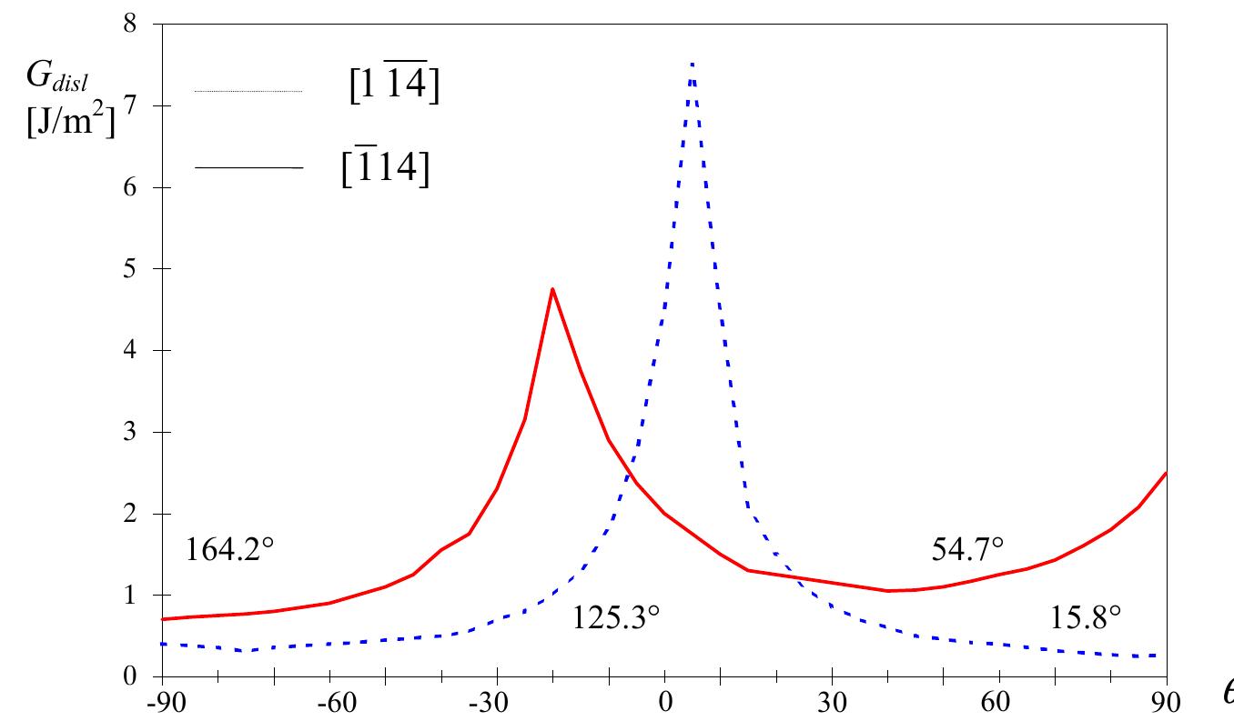
the (111) system are favorable for nucleation, so that @= 125.3°. From Eq. (57), energy release rate for positive [114] direction is Goi, = 0.86 J/m*. For (221 Jeu interface and negative [ 111) sli brittle in [114] crack direction, the active s pinSE angle y’=—79°, the system (111) are : (43), energy release rate for negative [ 114] direction is Gas) = 4.9 Jim’. ip systems have changed the (111 ) to the p plane with @= 54.7° and @= 164.2°, respectively. Due to the large negative Figs. 10 and 15 it may be conclud favourable for nucleation, so that @= 164.2°. ed that the cracking of copper bicrystals is a negative direction, while in Cu/sapphire bimaterials, cracking behaviour is he negative direction. As in bicrys als, Gas; is a function of @ but due to mode II loading conditions that are the most in the bimaterials, the minimum value occurs at arge values of @ angle, @= 130°. The minimum value of Gs; for bimaterials is much ower then for bicrystals. The phase angle effect plays an important role in bimaterial systems. The phase angle offect is shown in Fig. 16, which gives Gai; versus w’ for various slip plane inclination angles. Solid lines correspond to angles associated with direction [1 14 ] and dashed lines correspond to angles associated with direction [114]. Comparison of curves at y’= 0° and y’= 79° shows that favoured directions for dislocation emission reverse when the phase angle is altered. Crack tip fields for the crack along the interface between elastically dissimilar solids

the system is more likely to fracture by interface then substrate, and conversely. Comparing values of he energy release rate for the substrate or thin film with its values, one can define where the crack is going to propagate: into the substrate, into the thin film, or along the in factor, and mode mixity p erface. Values of the energy release rate, the stress intensity arameter can be determined in terms of only one dimensionless factor @, which is a function of sample geometry and materials elastic properties. The thin layers problem, under cond itions of residual tensile stresses, gives the appropriate model for solving problems in the area of composite materials manufacturing, electronic devices design, protective coatings problems, as well as for other applications.

Failure of component/structure can be attributed to numerous reasons, as showed in Fig. 1. Causes of failure shown in Fig. 1 can be classified in two groups, i.e. causes driven by design activities (positions 2 and 3) and causes driven by fabrication procedure in all positions 1, and 4 to 6). It can be concluded that major reasons for failure are to fabrication, service, and maintenance, i.e. activities depending on “human . This latter behaviour can be improved by implementation of quality assurance ter operating and controlling organization. On the other hand, about 29.3% of all failures are caused by poor design or standards. Therefore, this segment was in the focus arch, primarily due to high price of very responsible constructions (nuclear and plants, space and air industry, military applications).

The first and the oldest type of steel used as structural steels are plain carbon steels. The increase in strength was based on increase in carbon content. Carbon in Fe is a solid solution, with limited solubility. During deformation, as a result of applied stress, disloca- tions through their movement interact with obstacles, what in turn requires increase of applied strength for further deformation. Influence of carbon content on transition temperature in carhon cteele ig chown in Fico 2 [45].

Figure 3. Influence of sulphur content on transition temperature in steels [2]

ins as Manganese is substitutionally soluted in Fe, but the effect on strengthening is not pro- nounced since it depends on differences in atomic size. Mn and Fe are neighbouring elements in the periodic table. In structural steels, the content of Mn is in most cases limited to 1.5—1.7%, while larger content leads to increase of A,3 temperature and nuclea- tion of pro-eutectoid ferrite [6]. In other steels, the Mn content may be as high as 12%. The influence of Mn on transition temperature in C-Mn steels is shown in Fig. 4, [7]. Increase of Mn content decreases transition temperature to very low temperatures. The main mechanism lies in the sulphur have strong chemical affinity, leading to s during solidification of steel. solution is the addition of suf! formation of MnS The simplest way and tempered steels. During further metal working, MnS inc ed (rolling) or fractured and d ispersed (forging). Presence of sions in as-rolled steels is very dangerous, since the edges be manganese-sulphide). Manganese and pontaneous formation of MnS inclusion o completely remove S from the solid ficient amounts of Mn. This ro rise in toughness in low carbon steels, with excep e of Mn ensured significant ions in some medium carbon quenched usions can become elongat- long elongated MnS inclu- have as stress concentrators, leading to fracture or to lamellar tearing in welded constructions. The next task was to eliminate sulphides as critical particles. The solution was add itionally alloyed with Ca or rare earth elements (RE). This improvement was directly based on knowledge provided by fracture mechanics, i.e. addition of Ca primarily influences the shape of MnS. This feature is shown in Fig. 5 [1].

Figure 5. Shape of MnS after rolling (RD-rolling direction): (a) no Ca added; (b) addition of Ca [1] The next problem steel producers faced was the presence of free oxygen, originating from air blowing in converter, or in furnace. In order to eliminate oxygen it was necessary o modify the chemical composition by adding a specific chemical element with strong iffinity to oxygen. The answer came from the diagram of stability of oxides. Usually, Si or Al were used in an amount, estimated from the last chemical composition analysis Juring steel production (ladle after converter). This procedure introduced a new type of steels, so called killed steels, since oxide formation prevents bubbling of liquid metal. Furthermore, addition of Al became more interesting due to some observations showing hat in some Al-killed steels at grain boundaries precipitation of AIN occurred, decreasing srain boundary mobility. This was observed in steels in which Al was added in high amount; air-blowing (instead of oxygen, nowadays) led to reasonable presence of nitro- sen and strong affinity between Al and N. This was the first empirical case of grain ooundary control, but significant industrial application did not follow. On one hand, ohysical metallurgy defined mechanisms of deformation strengthening and recrystalliza- ion, and on the other hand, it has been a great effort to choose elements from the periodic able that behave similarly to Al, but with much better control. At firet an the lahnaratary ceale and later an fill indiuectrial ecale camnletely new Figure 5. Shape of MnS after rolling (RD-rolling direction): (a) no Ca added; (b) addition of Ca [1] After rolling, MnS becomes elongated, with very sharp tip. This shape leads to beha- fiour close to stress concentration. On the other hand, in Ca-treated steels, during solidifi- ‘ation, MnS starts to grow spherically. During both hot and cold deformation, due to 1igher Young’s modulus, Ca treated particles remain spherical. This approach has been -ver since of great practical importance, since it has focused attention on particle shape nstead on the overall level of impurities. Therefore, since spherical second-phase yarticles are not critical for stress concentration, toughness is improved, without any nfluences on other mechanical properties. In modern structural steels, sulphur content is ‘lose to 0.0050%.

Figure 6. Chronological development of the use of microalloying (MA) elements in steels [8] The main motives for developing MA steels were: significant increase in strength, resulting in either lowered construction weight or increased carrying capacity; thermo- mechanical treatment, a demand on the world market for steels with good weldability for pipelines, for which was not possible to use the “traditional” way to increase strength and toughness by heavier alloying- and carbon content. The microstructure of MA steels after hot working is typically fine-grained and consists of small and homogenous ferrite (@) orains. Small amount of cementite is also present (low pearlite steels are also used), together with fine dispersed carbonitride particles that can be observed only on electron microscope. The influences of niobium content and grain size on transition temperature in microalloyed steels are shown in Figs. 7 and 8, respectively. Theoretically the hest cqgmbination of strenoth and tonohness is ohtained in fine orain-

Figure 7. Influence of niobium content on transition temperature in steels [9] Figure 8. Influence of grain size on transition temperature [10]

Figure 11. Schematic interrelationship between the yield strength and the transition temperature T>7 for different steels [14]

Figure 12. Change of carbon content in structural steels during its development, [15°

Figure |. Net-section stress at instability vs. crack length for 7075 alloy T 6, [2)

T he results in Fig. 2 [2] show a large variation in toughness for experiments carrie out with an aluminium alloy (7075-T6) of different specimen thickness. Three regions i the toughness curve: A, B, and C can be recognized, taking into account the fractu profi tures es and stress-displacement curves form obtained in each region (Fig. 2b). The fra are Classified as “slant” or “square”, depending on whether the macroscopic fractui surface is at 45° to the tensile axis or normal to it. The second curve in Fig. 2a indicat how he proportion of square fracture varies with specimen thickness: up to the maximu! of the toughness curve (region A) fractures are completely slant, in thick specimens (regic C) they are generally square, and for intermediate thickness, they are of ‘““mixed-mode’’.

a 9 In region C (Fig. 2), specimens are rather thick so that all the load-bearing cross- section deforms in plane strain. Fracture propagates in the centre under critical crack tip conditions and any differences in behaviour of the specimen edges are insignificant in determining failure conditions for the specimen as a whole. Load increase is linear until a critical (low) value is reached, when fast failure occurs. The fracture of very thick speci- mens, region C, occurred with total instability at loads corresponding to a virtually con- stant toughness value and fracture appearance is almost completely square, with very small proportions of slant (“shear lips”) at the edges. The central region of a thick test- piece deforms under approximately plane strain conditions (Fig. 3). Then, the strain in thickness direction is zero, and when yielding occurs around a crack tip, high constraints are set up, and a triaxial stress state develops. This stress state enhances the initiation of fracture. The high value of maximum tensile stress below the notch may promote any cracking mechanisms to which the material is prone. If crack extension occurs when the strain in the region immediately ahead of the crack tip achieves a critical value, an effect of triaxial stress can arise through changes that it may make on the strain gradient in this region. For a given crack opening displacement, the plastic zone size in plane stress (specimen edges) is much larger than in plane strain (specimen mid-thickness), since yield- ing spreads under a shear stress component which includes full value of local tensile stress.

and dragging the slant (shear lips) with it. It is important to realise that, as the crack grows under increasing load, the plastic zone ahead of the crack tip grows bigger and is therefore more easily able to relax the through-thickness stress. Less of the thickness therefore deforms in plane strain and the proportion of square fracture decreases. At the thin end of the range, the initial square fracture occupies only a small proportion of the thickness cross-section; as it tunnels for- ward, the plastic zone size becomes large with respect to plate thickness; the through-thick- ness stress is relaxed; and final instability is achieved at a load, Fr, large enough to operate a sliding mechanism for separation, analogous to that in region A. The sequence of events illustrated in Fig. 4 is quite consistent, both with fracture appearance of broken specimens and with the observed load—displacement records. The fracture load is lower than that for a thinner specimen, because the testpiece, at instability, contains a longer crack.

initial ligament value. Bend angle is designated by @ and the value r(W-— a), added to crack length a, determines the actual rotation centre. The value of crack mouth opening displacement (CMOD), designated by 2v,,, is measured by positioning of clip gauge in knives of thickness z. The next analysis enabled to define crack tip opening displacement CTOD), for which symbol dis accepted. For known size of initial crack a and CMOD value, the answer whether fracture will take place before or after full scale yielding can be obtained according to ligament size (the distance to opposite side from crack tip). If he ligament is small, plastic zone will be formed across it before critical value of COD 0.) at crack tip is reached and fracture is ductile; if ligament is large, critical value ©, is reached first (before net section yielding) and fracture is brittle. Since in both cases the value of COD is almost the same, it is possible to use COD as a crack parameter.

Figure 6. The components of elastic stress field ahead crack tip

Figure 7. Modes of crack front displacement opening (1), sliding (ID), tearing (IIT) aS eae a, i, as Cottrell defined critical crack opening displacement 6, for plane stress condition and Vode I loading in the form:

In Eq. (7) the coefficient @= 1 for plane stress, and @= (1/3 to 1/4) for plane strain. Figure 9. The scheme of plastic deformation development around crack tip in a central part of the specimen for different load levels I-Initial stage (1-plastic zone, visible after unloading); II—Stage of relaxation (relaxed residual stress around crack tip); IJ—Blunting of a crack and small plastically deformed zone (2); 3 is the region in which material behaviour is described by K; value; I[V—Stable crack growth (4-zone of elastic unloading; 5-process zone; 6-Hutchinson-Rice-Rosengren zone; 7-zone of large plastic defor- mation, for net section yielding)

SoNtEG I Pip. 12 aS POSiwONned ON SUpPpOTts OF Ne tesunp Machine. The testing machine must be equipped with automotive device for load recording. Specimen holders have to assure minimum wear. Modern machines are designed in closed loop that enables load, displacement, or strain control and automotive recording of load, load line displacement, and crack opening displacement. The loading rate is limited 10 0.55—2.75 MPaVm/s. Crack opening displacement clip gauge design is recommended in standards. Recommended design comprises strain gauges of 500 ohm in Wheatstone bridge. It can be positioned on knives, joined to the specimen, or on machined holders ‘Fig. 13). Other clip gauge designs are also applicable. but strict linearity is required. 5. SPECIMENS FOR FRACTURE TESTING

Figure 14. Basic fracture mechanics specimen shapes and their marks

Figure 15. Marking of cracked specimen position in a material of rectangular and circular cross- section: a) specimen (and crack) position coinciding with main material directions; b) specimen inclined to main material directions; c) specimen from the circular cross-section material (L—direc- tion of grain elongation; C—circumferential or tangential direction; R-radial direction)

Figure 16b. Additional crack elements of flat specimens under loading effect: base points indicate fatigue crack tip before frac- ture testing; o—radius of blunted crack tip; 6,-crack tip opening displacement; a@-crack surface angle; vcrack opening displace- ment: o,-tensile stress component Figure 16a. Elements of an ideal through-crack in a flat specimen: 1—front crack surface (front plane); 2-side surfaces of specimen; 3—front of notch; 4— front of ideal crack; 5—front of real crack; 6—crack plane; 7—specimen crack plane cross-section; 8— front of side notch; 9-back specimen surface are uneven and, depending on their initiation and growth, they can have larger or smaller roughness. Such a crack is not suitable for analysis, so the term “ideal crack” is intro- duced, defined as a mathematical crack. In the unloaded state it has two separated, smooth and overlapped facing surfaces in the same plane (the crack plane) xOz (Fig. 16a), connected at the smooth line-the crack front. The front of an ideal through-crack is a straight line, or semi-ellipse or ellipse of surface- and embedded cracks, respectively. In the loaded specimen additional crack elements will appear (Fig. 16b). Cracks defined in this way enable mathematical analysis of fracture mechanics parameters.

wise the crack may deviate from that plane and the test result can be significantly affected. The K calibration for the specimen, if it is different from the one given in this test method, shall be known with an uncertainty of less than 5%. Fixtures used for pre- cracking should be machined with the same tolerances as those used for testing. The fatisue nrecrackings shall he conducted with the snecimen fullv heat-treated to the

Figure 19. Fatigue crack starter notch configuration

Figure 20. Envelope of fatigue crack and crack starter notches

For easier testing evaluation, the standards provide basic diagram forms, which can be obtained during the testing of fracture mechanics parameters. The six typical diagrams load vs. displacement (crack opening or load line), defined in BS 7448, are given in Fig. 21. First three diagrams, (1), (2), (3), because of total or most linear dependence of force F and crack opening V (i.e. load line displacement qg) can produce a valid plane strain fracture toughness result Kj.. Diagrams (4), (5), (6) correspond to the highest values of elastic-plastic fracture toughness (CTOD or J). The characteristic of plane strain fracture toughness is brittle material behaviour, so the appropriate load for calculation, Fo, is determined according to diagrams given in Fig. 22. First, the secant line is drawn, whose slope determined by quantity d, 5% lesser than the starting slope of the F—V diagram, i.e. only 4% lesser on the F—q diagram for bend specimens. Load F is the highest load recorded before Fz for type I and II dia- grams, and corresponds to the force Fy for a type III diagram. If the F,a,./Fo ratio is lower than 1.1, the Kg is calculated, competent to assess plane strain fracture toughness. If that ratio is greater than 1.1, CTOD or J should be determined as a fracture mechanics para- meter, as for type (4), (5), and (6) diagrams, shown in Fig. 21.

Figure 22. Determination of a appropriate load for calculation of plane strain fracture toughness RBIS RESID, ST Rn rene ESERIES ee Weisser eae ww ne Sine ene eww vines Ripe bs BBR BER BEE nee amon: SSESRRAIIN Nienvs Snows Nenenets SRTEAER Snes Werurn sn Nensteens Bente way BR Men wes ines SMtnnieontncnenaent “Swaninnnnnwnsesmewen omaavent? Men weng@@l pent eerneeanen lentes On diagrams in Figs. 21 and 22, the crack opening, i.e. notch opening displacement V or load-line displacement g are recorded on x axes. Subscript c (in V, g.) indicates brittle fracture or pop-in if Aa is lesser than 0.2 mm. Subscript m (Vin, Gm) indicates that max1- mum load level is achieved for the first time for general yielding. Subscript p indicates he plastic component, which corresponds to F,, F, or F', (Fig. 23). Subscript u indicates brittle fracture or pop-in for Aa greater than or equal to 0.2 mm. The same subscripts are also used to indicate appropriate crack-tip opening values CTOD (06), and the J integral. Calculation of an appropriate crack opening value dO requires determining appropriate oad F' and opening displacement V values. For diagrams (1) through (5) in Fig. 21 these values are (F., V.) or (F,,, V,.), depending on whether Aq is lesser (subscript c), or greater, ne: women ox fon lowe ao) 8 wens wad socom ace

Figure 26. Effect of temperature on the selection of proper fracture mechanics parameter

The most accurate crack measuring is when the crack plane surface area is divided by specimen width. It is enough to measure the crack length in 9 equally placed positions (Fig. 27). Initial crack length a, of SEN(B) specimen is the distance from the specimen surface to the tip of the fatigue pre-crack, while for a C(T) specimen it is the distance from the holder axis to the tip of the fatigue pre-crack. Crack length is calculated as the sum of average measurement at points 1 and 9 and the average of the remaining seven points (Fig. 27). Except force and displacement data, the calculation of fracture mechanics parameters requires crack data: initial fatigue pre-crack length, stretch zone (blunting), and crack growth (Fig. 27). These values can be determined after testing and final specimen frac- ture. If unstable fracture has occurred while testing, i.e. if the specimen was broken during the test, initial crack length and stable crack growth are measured. The final crack front is marked by additional fatigue of the specimen with the ratio

Figure |. Engineering stress-strain curve

Table 1. Typical values of modulus of elasticity at different temperatures The slope of the initial linear portion of the stress-strain curve is the modulus of elasti- city, or the Young’s modulus. The modulus of elasticity is a measure of stiffness of the material, for computing deflections of beams and other members. However, an increase ir temperature decreases the modulus of elasticity. Typical values at different temperatures are given in Table 1, [3].

Figure 4. Comparison of stress-strain curves for high-and low-toughness materials The toughness of a material is its ability to absorb energy in the plastic range. The ability to withstand occasional stresses above yield stress without fracturing is particular- ly desirable in parts such are freight-car couplings, gears, chains, and crane hooks. Toughness is a commonly used concept which is difficult to pin down and define. One way of looking at toughness is to consider that it is the total area under the stress-strain curve. This area is an indication of the amount of work per unit volume which can be done on the material without causing it to rupture. Figure 4 shows stress-strain curves for high and low-toughness materials. The high-carbon spring steel has higher yield- and tensile strengths than the medium-carbon structural steel. However, the structural steel is more ductile and has a greater total elongation. The total area under the stress-strain curve is greater for the structural steel, and therefore it is a tougher material. This illustrates that toughness is a parameter which comprises both strength and ductility. The crosshatched regions in Fig. 4 indicate the modulus of resilience for each steel. Because of its higher yield strength, the spring steel has greater resilience.

The engineering stress-strain curve does not give a true indication of deformation characteristics of a metal because it is based entirely on original dimensions of the specimen, and these dimensions change continuously during the test. Also, ductile metal pulled in tension becomes unstable and necks down during the course of the test. Since he cross-section area of the specimen decreases rapidly at this stage in the test, the load required to continue deformation falls off. The average stress based on original area decreases likewise, and this produces the fall-off in the stress-strain curve beyond the point of maximum load. Actually, the metal continues to strain-harden all the way up to fracture, so that stress required to produce further deformation should also increase. If rue stress is used, based on the actual cross-section area of the specimen, it is found that he stress-strain curve increases continuously up to fracture. If the strain is measured also instantaneously, the curve which is obtained is known as a true-stress—true-strain curve, or a flow curve. Any point on the flow curve can be considered as the yield stress for a metal strained in tension by the amount shown off the curve. Thus, if the load is removed at this point and then reapplied, the material will behave elastically throughout the entire range of reloading. Figure 5a shows the flow curve for a rigid, perfectly plastic material. For this idealized material, a tensile specimen is completely rigid (zero elastic strain) until axial stress equals o,, whereupon the material flows plastically at a constant flow stress zero strain hardening). This type of behaviour is approached by a ductile metal which is in a highly cold worked condition. Figure 5b illustrates the flow curve for a perfectly plastic material with an elastic region. This behaviour is approached by a material such as plain carbon steel which has a pronounced yield-point elongation. A more realistic approach is to approximate the flow curve by two straight lines corresponding to the elastic and plastic regions (Fig. 5c).

In Fig. 6, the true-stress—true-strain curve is compared with its corresponding engi- neering stress—strain curve. (Because of relatively large plastic strains, the elastic region has been compressed into the y axis). In agreement with Eqs. (2) and (4), the true-stress— true-strain curve is always to the left of the engineering curve until the maximum load is reached. Beyond maximum load, the high localized strains in the necked region, Eq. (15), exceed the engineering strain calculated from Eq. (2). Some flow curves are linear from maximum load to fracture, in other cases its slope continuously decreases up to fracture.

Table 2. Values for n and K for metals at room temperature [4] 2. IMPACT TESTING

the fracture surface that is cleavage (or fibrous) fracture. Figure 10 shows how the fracture appearance changes from 100 percent flat cleavage (left) to 100 percent fibrous fracture (right) as the test temperature is increased. The fibrous fracture appears first around the outer surface of the specimen (shear lip) where the triaxial constraint is the least. Gradual decrease in the granular region and increase in lateral contraction at the notch with increasing temperature is visible. Sometimes in the Charpy test the ductility is measured as indicated by the percent contraction of the specimen at the notch.

Both tested materials are of the same absorbed energy in temperature interval —140°C to +20°C, having the same ratio of crack initiation to crack propagation energy at room temperature (Fig. 14). However, this ratio is different for the same total absorbed energy. Crack initiation energy is always lower compared to crack propagation energy in case (a). whereas this relation is changed in case (b). This behaviour has to be appreciated when evaluating the use of material at low temperature and at high load rates.

Figure 14a. Different shapes of diagrams for Charpy test at different temperatures

The significance of impact testing is illustrated by test results for two high strength steels presented in Fig. 15. Chemical composition is given in Table 3, and tensile proper- ‘ies in Table 4. The difference in strength and ductility is not expressed in the same level as the case with impact toughness properties. Steel A, with low carbon content, exhibited high impact energy at low temperatures (down to —100°C) for crack propagation and also crack initation [8]. However, there is a significant effect of rolling direction. For steel B, with 0.3% C, the impact energy is low, and nil ductility transition temperature can be determined (between —40°C and —60°C).

Table 3. Chemical composition (wt%) of tested steels Table 4. Tensile properties of tested steels

Probably the chief deficiency of the Charpy impact test is that the small specimen is not always a realistic model of the actual situation. Not only does the small specimen lead to considerable scatter, but a specimen with t constraint as would be found in a structure wi hickness of 10 mm cannot provide the same h much greater thickness. The situation that can result is shown in Fig. 16. At a particular service temperature the standard Charpy specimen shows a high shelf energy, while actually the same material in a thick-section structure has low toughness at the same tem problem is the development of tests that are perature. The most logical approach to this capable of handling specimens of extended thickness (e.g. explosion bulge test, drop weight test).

Figure 18. Explosion bulge test, developed in the U.S. Naval Research Laboratory (NRL) In addition to fast fracture by explosion shot, a unique “crack-starter” can contribute to brittle fracture condition. In the first development [10] of explosion bulge tests the test plate was supplied with brittle weld bead deposited on the surface of 25 mm steel plate, sized 500x500 mm. The latter feature is a short bead of very hard brittle weld metal which is notched in a manner to insure the initiation of a cleavage crack as soon as the base metal is subjected to any bending. The specimen, with the welded short bead face down is placed upon the circular supporting die and a standardized charge of explosive is detonated at the fixed position above the specimen. During the extremely rapid loading, he brittle weld bead introduces small natural cracks in the test plate (similar to a crack in weld), initiating cleavage cracks at the root of the notch and transferring them to the base metal as running cracks. The behaviour of the test plate depends upon the ability of the base metal to arrest the running crack and to deform while permitting only high-energy absorbing, shear-type fracture to propagate. If the steel is not capable of arresting the running crack, the plate develops many cleavage fractures and breaks flat; that is, little plastic forming occurs downward into the die cavity. Tests can be carried out over a range of temperatures and then the appearance of the fracture determines the transition tempera- tures (Fig. 19). Below the NDT the fracture is a flat (elastic) fracture running completely to the edges of the test plate. Above the nil ductility temperature a plastic bulge forms in the center of the plate, but the fracture is still a flat elastic fracture out to the plate edge. At a still higher temperature the fracture does not propagate outside of the bulged region. The temperature at which elastic fracture no longer propagates to the edge of the plate is called the fracture transition elastic (FTE). The FTE marks the highest temperature of fracture propagation by purely elastic stresses. At yet higher temperature the extensive plasticity results in a helmet-type bulge. The temperature above which this fully ductile tearing occurs is the fracture transition plastic (FTP).

In this way welded joint specimens could also be tested (Fig. 20).

The explosive charge capacity was selected for loading the specimen to insure a con- tinuing store of energy to feed the propagating cracks. In essence, the gas pressure was maintained for sufficient duration so that stress unloading could not occur during crack- ing. The final feature of the explosion bulge test is to have a series of specimens heated or cooled to progressive temperatures over a range that encompasses expected fracture tran- sition points (Fig. 19). Welded joint (and unwelded) test plates are notched in the bead of brittle weld metal to provide small flaw and are subjected to repeated shots. Weld rein- forcement on face is ground flush at end to permit notch depth developement without visible intimate contact with supporting die. Below nil ductility temperature, the test plates show no deformation because the weld crack is accepted by the base metal (starting in the heat-affected zone) as a brittle running fracture, and is unable to resist its propaga- tion by cleavage fracture. Above this transition temperature range, the brittle weld crack is arrested. Energy from the explosive charges is effectively utilized by the plate, by successive bulging into the die. Plate thickness in bulge is measured after each shot. The explosion bulge test makes use of a large plate specimen that incorporates novel features in its preparation and testing procedure. However, the application of explosion in

Figure 21. Typical results of explosion bulge test for steels A and B, expresed by reduction of thickness AR and bulge development B vs. number of explosions L-notch in hard bead in cross-rolling direction; C—notch in rolling direction

3.2.1. Determination of nil-ductility temperature from tested specimens imposed stress in the outer fibers rises to the yield point, the steel either (1) accepts initia- supported as a simple beam. The brittle weld bead as a result of dynamic loading from a falling weigh is fractured at near yield-s ion of a cleavage crack which “runs” completely through the section and results in a broken specimen (Fig. 25), or (2) initiation of cleavage fracture is resisted and men bends the small, additional amount permitted by the anvil stop, withou fracturing. The specimen, before testing cooled in a bath to the requested tem the speci- t complete perature, is ress levels . If the starter-crack propagates across he width of the plate on the tension surface to the edges, the test temperature is below the NDT. Complete separation on the compression side of the specimen is not required. The ity break is produced. The test is quite reproducible and NDT temnerature in this test can be determined to the nearest — 12°C. NDT is the highest temperature at which a nil ducti Figure 25 provides essential details of the bead-on-plate specimen with the “crack- starter” weld, and the procedure which is employed to test a series of specimens over a range of progressive temperatures to determine the NDT for steel. The drop-weight test was devised for testing relatively heavy structural sections, and is not recommended for base metal pieces less than 12.5 mm thick. A complete description of the standard method for conducting the NRL Drop-Weight Test is presented in ASTM E 208. A specimen is considered broken if fracture on tension surface extends to one or both

Figure 25. Results of drop-weight test for determination of nil-ductility transition temperature

Figure 26. Dynamic drop-weight tear test Figure 27. Robertson crack-arrest test

Figure 27. Temperature dependence of yield strength (,), tensile strength (0,,), and fracture strength for a steel containing flaws of different sizes More detailed consideration is necessary before use of transition points in engineerin design through the fracture analysis diagram, through reference to basic properties of th tension test. The sub-ambient temperature dependences of yield strength o, and ultimat tensile strength o, in a bcc metal are shown in Fig. 27. For an unnotched specimen with out flaws, the material is ductile until a very low temperature, point A, where o, = o, Point A represents the NDT temperature for a flaw-free material. The curve BCD repre sents the fracture strength of a specimen containing a small flaw (a<0.1 mm). Th temperature corresponding to point C is the highest temperature at which the fractur strength o;» o,. Point C represents the NDT for a specimen with a small crack or flaw The presence of a small flaw raises the NDT of a steel by about 90°C.

Figure 28. Fracture-analysis diagram showing influence of various initial flaw sizes [13] C- f+ & Data obtained from the DWT and other large-scale fracture tests have been assembl by Pellini and co-workers [13] into a useful design procedure called the fracture analys diagram (FAD). The NDT as determined by the DWT provides a key data point to ste onstruction of the fracture analysis diagram and transition temperature features of stee (Fig. 28). For mild steel below NDT the CAT curve is flat. A stress level in excess of : to 55 MPa causes brittle fracture, regardless of the size of the initial flaw. Extensi Sorrelation between NDT and Robertson CAT tests for a variety of structural steels hav shown that the CAT curve bears a fixed relationship to the NDT temperature. Thus, tl NDT -—1°C provides a conservative estimate of the CAT curve at stress of 6,/ NDT +15°C provides an estimate of the CAT at o= 0, and, the FTE and NDT +50° provides an estimate of the FTP. So, once NDT for structural steels is determined, tl entire scope of the CAT curve can be established well enough for engineering design.

Figure 30. Application of DT test results for fracture analysis diagram design Fig. 30, using NDT as base (dashed line). Below the NDT the fracture is brittle and has a flat, featureless surface devoid of any shear lips. At temperatures above NDT there is a sharp rise in energy for fracture and th fracture surfaces begin to develop shear lips. The shear lips become progressively mor« prominent as the temperature is increased to the FTE. Above FTE the fracture is ductile void coalescence-type fracture. The fracture surface is a fibrous slant fracture. The uppe: shelf of energy represents the FTP. The lower half of the DT energy curve traces th emnperature course of the CAT curve from NDT to FTE.

ee eae Me, ee! ae ee eee, San Loe ir meena Meee a The most common forms of material failures are fracture, corrosion, wear, and defor- mation. Before the actual failure mode can be determined, however, a failure analysis must be performed. In order to analyse a failure, circumstance analysis is required follow- ed by chemical analysis, mechanical properties and microstructural analysis. Fractogra- phic analysis, Fig. 1, often has the most dominant role in analysis of failure of metal parts and constructions, [1]. me: a ~~ - € we Uté<‘<‘ we x om: » » se

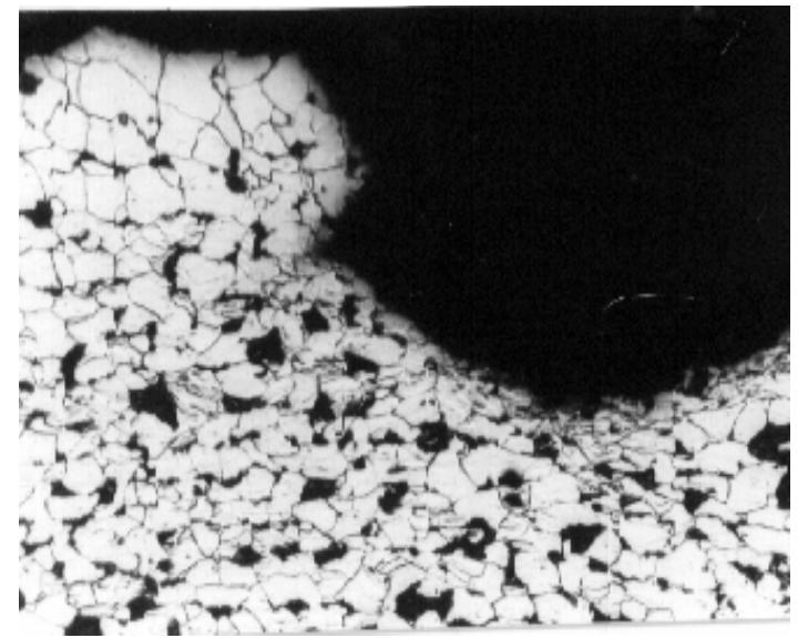
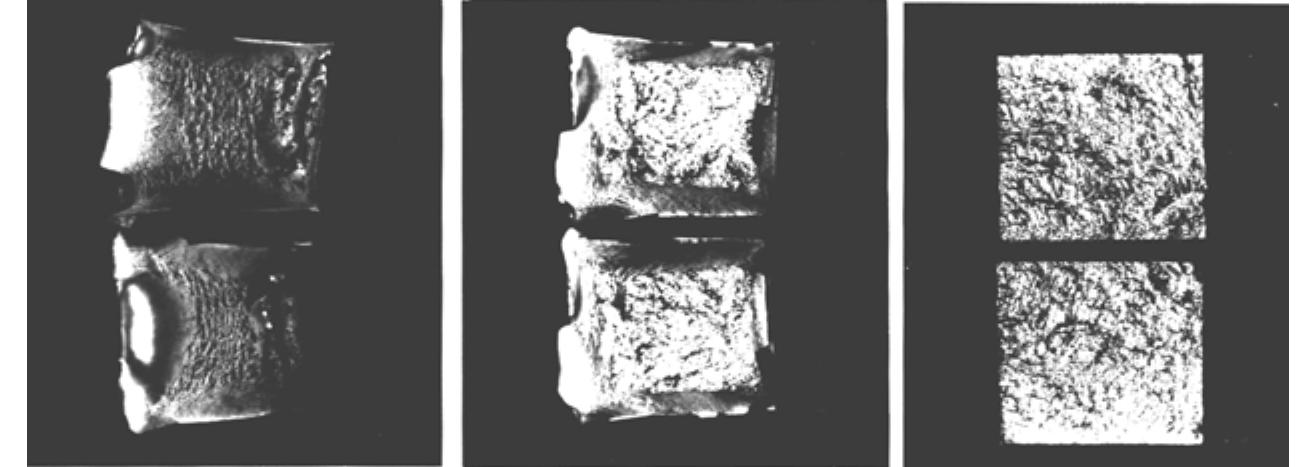
During welded joint testing, a vast number of macroscopic cracks had been detected. The first step was to take samples with the cracked material, positioned in liquid and gas phases of the sphere. In the next step, the small “boat” type specimens from meridian and equatorial welds were prepared, Fig 3. The crack, several centimetres long, was discover- ed in the equatorial weld, propagating in the heat affected zone, Fig. 4. Fractographic analysis was difficult due to corrosion of the fractured surface, and it was impossible to make reliable conclusions about the cause of failure. 3.1. Fracture analysis of the heat-affected-zone For better and easier examination of the cause of welded joint failure, simulated welc ing on the same steel was performed. The microstructure of different temperature region in HAZ had been simulated on the Smitweld LS1402 device. The samples, 60 mm lon; 11 mm wide, and 11 mm thick, had been exposed to different temperatures: 1350°C -orresponding to coarse grain formation; 1100°C — fine grain formation; 950°C — fin srain region above A,3 tempera ransformation of austenite, be 800°C to 500°C of 15s was co esting was performed with C Jepth. The fractured surface of Charpy specimens was analysed by scanning electro microscopy, JEOL35, [2]. Regions corresponding to d ure — austenite-ferrite transformation; and 850°C — par harpy specimens (10x10x55 mm) with a 2mm V no tween temperatures A,; and A,3. The cooling time fror nstant, selected as typical for tested steel welding. Impac ifferent simulation temperatures are shown in a welde le Cc

Figure 5. Scheme of welded joint and heat affected zone with macrofractographs of specimens simulated a) 1350°C, b) 1100°C, c) 950°C d) 850°C (10x)

Figure 9. Schematic representation of quasi-cleavage

Microvoid coalescence, or dimple fracture, usually occurs under single load or tearing. [his is shown by depressions in the microstructure called dimples, which occur from nicrovoid emergence in places of high local plastic deformation. Under increased strain, nicrovoids grow and coalesce until rupture occurs, thus dimple rupture. Dimple size and shape depend on the type of loading and extent of microvoid emergence. When a material s put under uniaxial tensile loading, equiaxed dimples with complete rims appear. Under 1 tear loading the dimples are elongated, the rims of the dimples are not complete and the limples are in the same direction as the loading. Shear loading has the same features as ear loading except the dimples are in opposite directions. Oval dimples occur when a arge void intersects a smaller subsurface void, the dimples form an oval shape and exhi- nit complete rims. A serpentine glide is an interwoven pattern of glide plane decohesion steps. Ripples are partially smoothed out areas of serpentine glide. A stretched area is a flat featureless area resulting from further straining of a ripple pattern. Intergranular imple rupture occurs along grain boundaries due to nucleation and coalescence of voids ut grain boundaries.

ULTACeSs Nave NUMCTOUS CUPIIKE GOpresslOns OF GUNIpIes . Until recently, dimples have been classically divided into three groups: equiaxe imples, shear dimples, and tear dimples. Schematic diagrams illustrating how these at onventionally formed are shown in Fig. 11. Equiaxed dimples do not always appez xactly equiaxed in SEM fractographs, because tilt angles of 30° to 45° are often used t rovide good contrast, and therefore the dimples may appear slightly distorted. Howeve he shear-lip zone of a Charpy impact, tensile-test, or fracture-toughness specimen wi lisplay a well-defined network of oval dimples elongated in the same direction — the direc ion of shear. With shear dimples, it is quite difficult to identify the site of microvoid initic ion, because the carbide particle or inclusion responsible may be hidden below the su ace which mav have heen rubbed or flattened out bv shear disnlacement during fracture.

Close examination of the initiation area reveals that initiation occurs at the point between two closely spaced particles, Fig. 13. Energy dispersive X-ray analysis (EDX) on the particles indicated that there was no inclusion. To identify these particles, the fracture surfaces were etched and re-examined in the SEM. Figure 14 shows matching facets after etching. The particles have the smooth and blocky appearance characteristics of M—A constituent and lie on a prior austenite grain boundary. Failure initiation has therefore occurred from between two M-A particles, in close proximity, located at the prior austenitic grain boundary. Figure 12. Second phase particles in the intercritically reheating coarse grain region microstructure: TEM and SEM micrograph of an M-—A particle

‘igure 13. SEM micrographs of matching facets showing the initiation site for the intercritically reheating coarse grain structure

Figure 14. SEM micrographs of etched matching facets showing the initiation site for the intercritically reheating coarse grain structure

The introductory short story is representative for the related developments and genera importance of fracture mechanics application in the scope of structural integrity. During pull-up at Air Force Base, Nevada, December 1969, an F111A (Fig. 1) experi enced catastrophic failure of the left wing, causing the destruction of the aircraft and th death of the pilot. The failure initiated at a pre-existing manufacturing flaw due to a forg ing fold in a critical wing pivot fitting in the high strength D6AC steel forging. The flav had passed undetected through inspections and grew to critical size when the airplane ha accumulated only 105 flying hours, although the fatigue life was estimated to be abou 10,000 flight hours. The F111 had been based on the safe life design philosophy, developed after the war years in an effort to take into account cyclic stresses that lead to fatigue of airframes. The approach is similar to the conventional engineering method of stress allowable, based on the maximum stress that can be permitted in a material for a given design condition to prevent failure. Materials allowable were obtained through a testing program. Addition- ally, the safe life approach involves rigorous fatigue testing of a full, representative 1irframe assembly for 40 000 hours ensuring a safe life of 10 000 hours. The safety factor of four was o take into account unknowns, assumptions and variables applicable to the fleet as a whole. Unfortunately, while this approach proves the overall airframe design for a certain safe fatigue life, it does not take into account the effect of a single trivial defect, nowhere to be found by non-destructive inspection (NDI), introduced in a particular 1irframe at manufacture. Thus, the overall design may be acceptable respective require- ment, but unforeseen small random flaws can undermine this and cause failures, well below the safe life, as it had occurred. ; a: ee ee: ee a i a ee ee ee ee: A me oa: :, ee

deterministic approach the Safety Factor is the ratio of material strength and the stress Caused or ave of pro centra with a part. I selecti safety safety is rea on of t by the limit load. In rage values of both p bability, Fig. 2. The resulting values will be then very different in dependence ot he proposed reliability. Of he combination of actual s factor, 50% of factor below t ly possible tha part will prematurely fail (s he safety factor, so to allow for the allowable stress to be at the “minimum’ of expected values. Accord values COITes pond to the va (with a confidence level of based on actual stress and s the 99% grou the probabilistic approach this factor is the ratio of the mear arameters (“central safety factor”) or connected to any value interest is that for a particular part the actual safety factor, as ress and strength, is not known. We know that in case of ¢ all parts have the safety factor above this value, and 50% are his value. But we do not know how to classify this particula1 the safety factor for a particular part is below 1 and that this haded area in Fig. 2). This usually results in the conservative ing to the MIL-Handbook, for example, A-basis allowable ue for which at least 99% of the population have to survive 95%). Also in this case the particular component may be, as rength combination, far above the allowable (if it belongs tc p) or below (belonging to the 1% group).

For typical engineering materials with average ductility, the effect of the crack-like defect should not be forgotten and conditions for pure collapse do not appear. Starting from this presupposition, the new method has been developed by the author, and is based on approximation of stress-strain conditions (plasticity) in the net section weakened by the crack (geometry), and is successfully applied in the design of the ARIANE 5 rocket case and verified on two different materials. rm 1 . rMrA SL 1 ,° 1 1 ae | oar 1 3 mG

Figure 5. Building block verification strategy An analysis to determine stresses, resulting from combined effects of force, internal yressure and associated thermal gradient, is usually performed using finite elements valculation. This kind of analysis will usually assume no crack-like defects in the struc- ure. For an e all important structural phenomena are well understood and fully considered within geometrical and physical model. Typical step-by-step analysis procedure, based on U1 ding bloc fficient and accurate analysis, the complex operational environment requires ks, is the most adequate (Fig. 5). Well-executed finite element analysis can esult in saving money, time, and effort within the design process. The sense of exact ac -alculation, p ors, or in no sense ors are pu robabilistic consideration, and damage tolerance design is to reduce safety better use of available potential. On the other hand, a very exact calculation if the safety factors are unchanged, being the case if the selected safety rely empirical and not based on analysis and verifying experimental results.

Figure 6. Ductile tearing by hole growth and coalescence The integrity assessment of a cracked structure by conventional fracture mechanics is oased on a single parameter, supposing that it uniquely characterizes the material fracture ‘esistance. Under two-dimensional conditions (through crack defects) the parameter K;., is the stress-intensity value at the crack tip for unstable crack growth, is the fracture oughness for plane strain conditions, and is an inherent material property, while resis- ance to the onset of ductile fracture is characterized by a critical value of the J-integral, J,.. Because the micro-mechanisms of fracture require attainment of the critical condition, Jescribed in terms of stress or strain, different values of applied crack driving force may oe required to cause fracture in different structures. These interrelated effects of geometry and loading mode on near-tip stresses or strains, and fracture toughness, are referred as size effects. Early fracture mechanics research addressed size effects to establish size and Jeformation limits below which the geometry independence of fracture toughness is assured and a single parameter describes uniquely and completely stresses and strains near the crack tip. This enabled application of conventional single parameter fracture nechanics approximation to assess the fracture integrity of structures irrespective of the nicro-scale fracture mechanism. Testing standards, which govern the measurement of K,, and Jj., require sufficient specimen thickness to produce predominantly plane strain conditions and sufficient crack depth to position the crack tip in a highly constrained field. The requirements of the testing standards guarantee that K,, and J;, are lower bound, seometry independent measures of fracture toughness.

One of the most important contributions of fracture mechanics to structural integrity i the application in the study of crack growth. For technical materials, fatigue crack propa gation has been shown as crack extension during every load cycle by correspondin: striation development. The origin of striation is based on the plastic blunting process o the fatigue crack in each cycle. The example in Fig. 7 may help understand the concept o growing fatigue crack as related to da/dN values, presented by electron microscopic frac tography of a fatigue fracture surface. The number on the left indicates the number o cycles (striation) at each stress level. Figure 7. Fractographic view by electron microscope of a fatigue fracture surface

On the left end of the curve, the fatigue crack growth threshold is the theoretical value of AK at which da/dN approaches zero. However, relationships in this regime (A) are more complicated. A simple explanation would be that if the stress intensity range does not exceed AK,,, there would be no propagation of existing cracks. However this is only valid if the crack does not close, so that the stress intensity is AK = Kinay — Kmin. But if the crack closes at some K = Koy > Kinin (Kop 18 not a material parameter or constant and depends on the type and history of loading) this relationship is no more valid and the stress intensity range causing crack growth reduces to an effective value Ak —_ Y ye SPIN

Depending on the loading sequence, crack growth can be accelerated or decelerated what is known as load interaction or load sequence effects. More specifically, crack growth deceleration is known as retardation. Two kinds of ideas persist in literature regarding causes of the load interaction effect: based on plasticity-induced crack closure and based on the plastic zone ahead of the crack tip. In general, history effects can be rather pronounced in variable amplitude loading if the rate of stress intensity (dK/da) i: low or the variable amplitude loading is not confined to single overloads. In the latte: case, there are of course marked history effects, as long as the crack is propagating withir the plastic zone stemming from the overload. Luckily, simple fatigue laws, not taking retardation effect into account, are usually conservative. OW. 3: Gee ee ee ee, ee ee Oe NS Ae ee ee ee ee ae Due to relatively small differences, it is experimentally difficult to confirm existence of closure and quantitatively correlate with observed fatigue behaviour. Some may argue over this, because true effects of closure are negligible, but another problem may lie with inherent difficulties in measurements.

By introducing the above time dependent correction in the Strain Range Partitioning equation, excellent results have been achieved in life prediction of cyclic dwell history tests in the relevant temperature range 750° to 850°C, for the given alloy. Additional evidence about the accuracy of the developed method has been accounted for by investi- gation, prediction, and comparison of available literature data for the alloy 800 H. The method produces very accurate results for all data included in the analysis, covering a number of different material lots, treatments, and testing conditions. For practical application of the method, based on general time-temperature depen-

Figure 15. Proof test logic based on fracture mechanics guarantees that the required remaining life can be realized without incurring an unaccep- table risk of failure during proof. This test is not very useful if probability of failure is high. In general, the evaluation of a, is simpler than as, because conditions for the proof test are controlled and very well known, and also less complex than service conditions.

Figure 16. Scheme of the Leak-Before-Break procedure Component behaviour and relevant relationships can be presented in a simplified wa 1 the so-called rack depth a/t and critical surface crack half-length c/c,. Line AB de rack growth init 1e range of the t iation of a surface crack. The second vertical line with hrough-wall crack below and above critical crack lengt eak-before-break diagram (Fig. 16). Axes in the diagram are: relativ fines the place c c/c, = | separate h and in this wa} ne area of safety. It can be seen, however, that part-through cracks of length higher tha ~ may also be stable if their position is be racks grow furt roduce fracture, and the application of leak- econd example curve 2 in Fig. 16, arrow), t ow the ligament failure ine. But if thes her (Fig. 16, curve 1) due to fatigue or sustained crack growth, it wi before-break concept is not possible. In th he ligament line is first ac hieved and stabl sakage may appear if the crack grows along the surface up to the size where crac pening is sufficient for leakage to be discovered before critical crack size is achieved. | 1e crack growth path position is very near irection (arrow 3), the conditions of catastrophic fracture may also be possible. 0 c=c, and its shape cu rved in the sam

Figure 17. Creep curves for 2 4 Cr1Mo steel JODE-UINEe Values diG UsUdlly Ddsed OL UNCdr CAUAaPOAUOT OL CAPCTUMCHtal SHOTT- tune] data. The experience with old power plants showed however, that the deterministic life evaluation, applying the worst case assumption, pile-up conservative assumptions leading to the pessimistic assessment, different to the actual situation and shortening the life time. Typical creep results (Fig. 17) show that between allowable, minimal and mean values, significant life capacity exists compared to the design life, which is reached first. Although a large amount of reserve exists, in the particular case there are no quantitative data, and starting from the worst case assumption it will not be possible to use these capacities. Obviously, the solution of this problem, without negative effects on general safety and reliability of the equipment, is only possible using special methods to measure actual life consumption and remaining life capacity of parts in service and ruling out the corresponding random effect in this respect. Accordingly, from the design life calculation point of view, here is not a matter of correcting the errors in calculation and all strives of “Improvement” in this respect will not be successful. However, the modern method of life design certainly considers the corresponding experiences with the introduction of life monitoring and equipment inspection, contributing in this way to the overall efficiency and reliability of equipment. Programmes for monitoring and life extension are now usual in power plants. The goal of these programmes is the increase of availability, efficiency and reliability of existing power plants by reassessing their structural integrity and the es wesenenentcere aul cto. eeeael coveresreeeniewss | aaciererees

Table 1. Recommendations for different materials

Figure 18. Relation between area fraction of cavities and life fraction

Figure 19. Creep damage classes as seen from the replicas

Table 3. Possible causes for weldment residual stresses

Table 2. Functional classification of flaws 2. METHODOLOGY FOR DETECTING CAUSES OF MALFUNCTIONING

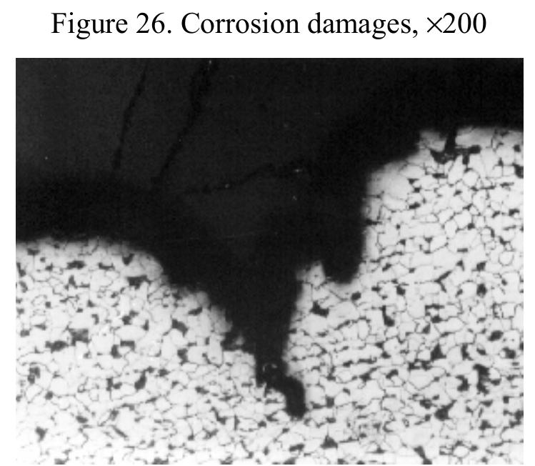
Te eee eee eee eater eee eer eee ee eee ee eee ee DE eee neon ae ee ee ee a The specimens for experimental investigation were cut from turbine blades, stator and rotors, Figs. 2-4, made of high-content chromium steel X22CrMoV121 (according t DIN standards), which fractured after less then half the predicted life time. These steel belong to the martensitic steel type, with 5% of maximal allowed 6-ferrite content anc which are highly used for turbine blades. The comprehensive experimental investigatiot of microstructure and fracture features 32 different specimens tested by optical micro scopy, scanning electron microscopy with energy-dispersive analyzer, all performed 11 the aim of determining microstructural variations, and their possible influence on fracture corrosion, and oxidation resistance of blades [13-15]. The basic microstructure of tested steels is martensite with carbides, separated in grai boundaries and within the grains, Figs. 5—6. In addition, an appearance of an extremel large amount of ferrite is detected. The various microstructural flaws already mentione are presented on SEM micrographs: the striped carbides distribution; the inhomogeneou distribution of chromium and the related inhomogeneous distribution of carbides i different zones; very large carbides of chromium, separated in grain boundaries wit decohesion in the particle—matrix interface; very long MnS inclusions passing throug several grains; massive silicon inclusions are also revealed. A relatively large number specimens have a martensitic—ferritic or pure ferritic structure with large chromiut carbides in grain boundaries instead of the necessary structure of tempered martensit Delaminations of microstructure are observed too, Figs. 7-12. As illustrated on the last four figures, the corrosion pits, because of the complex stres

Figure 13. Initiation of fatigue crack on corrosion pits’ Figure 14. Fatigue — striation

Figure 6 6. . Improper microstructure — martensite with inhomogeneous carbide distribution

Figure 15. Corrosion pits and cavities Figure 17. Scenario of failure

i Yiww Austenitic stainless steels are often used for welding or repair welding of dissimilar netal joints as a filler material. However, because of their coefficients of thermal expan- ion and low thermal conductivity, and high residual stresses and distortion being related o the same quantities of joined metals, many problems emerge during exploitation at levated temperature. Basic structures of austenitic steels are simple and several transfor- nation phases can be produced during welding that play a significant role in service vehaviour. Extensive transformation may take place during component life if it is main- ained at elevated temperature.

Figure 16. Cr — distribution in the corrosion pits

Figure 20. Austenitic weld zone. Stress corrosion crack. Precipitated carbides in grain boundaries and zone with- out carbides in the vicinity of crack Figure 19. Welding flaw in austenitic zone

Figure 21. SEM micrograph of austenitic-ferritic inter- face. Large crack, brittle intercrystalline fracture in aus- tenitic zone. Complex silicate inclusions

Figure 22. Macro photo of “window” type fracture with schematic view of the specimen

Figures 23 and 24. Cracks due to hydrogen damaging

Figure 25. Flow patterns during: a) transition boiling, b) local steam blanket formation downstream flow disrupter

Figure 28. Corrosion damage with sharp tip, x50

Figure 32. Main hot water pipeline Fig. 33. According to the design specification, magistral piping was made of seamed tubes, dimensions of ©4067 mm and covered with polyurethane. Detailed visual exami- nation and extensive destructive testing showed that frequent leakage of piping is due to design flaws and also due to technological and service flaws. It was established that the piping built-in thickness (approximately 4.5-5.5 mm) is considerably lower from the designed value, and thus qualifies as a technological flaw.

Figure 34. Damaged area due to leaking, wet insulation Figure 35. Misaligned welds with crack in common HAZ

Figure 36. Penetrated crack in HAZ where leaking occurred

Figure 1. F asa function of temperature T, for a carbon steel (1) and an austenitic steel (2) Clearly, for materials prone to embrittlement, one can expect still further decrease in fatigue crack size limits in view of such factors as hydrogenation, radiation, and corrosive effects. At the same time, in the case of austenitic steels and aluminium alloys, which do not embrittle at low temperature [1], the area occupied by a fatigue crack prior to fracture scarcely decreases with lowering temperature. A study of fracture of various engineering components and structures has revealed that in most cases their fracture is due to material fatigue, which is known to be responsible for initiation and propagation of fatigue cracks in cyclic loading and such cracks ultimate- ly lead to complete failure of a component. The most dangerous fracture case is where a component completelv fails with a

Table 1. Mechanical properties of the materials under study

Table 2. Fracture toughness characteristics

Figure 2. Comparison between fracture toughness characteristics under static and cyclic loading: (1) heat resistant steels; (2) chrome—molybdenum steels; (3) titantum alloys; (4) austenitic steel; (5) 20L steel. (Open and solid symbols indicate fulfilment or non-fulfilment of plane strain conditions, respectively; half-solid symbols correspond to the case where plane strain conditions were fulfilled in the K,, determination and not fulfilled in the Kg” determination.) YALIOUS DALCHes dll MWA suenuUy GQUIer it PrOperues, Figure 2 compares the static and a fatigue fracture toughness characteristic of the -onsidered materials, shown in coordinates Ky/Ko"""—Ko""’. This figure presents more lata than Table 2 because we additionally used the results for specimens: of various sizes 30,35,37]; tested at various stress ratios [29,33,35,40]; for plastically prestrained speci- nens [41-43]; specimens of titanium alloy with different content of nitrogen and oxygen mpurities [53]; and specimens of steel 20L after various service periods [56]. The results of investigation of the influence of these factors on fatigue fracture toughness will be liscussed in the next report.

“—-s values of the stress intensity factor are taken as Ky. Figure 3 compares Kj’ and K,, values for studied materials. It is evident that Kj’ is approximately 20% lower than K;,., and scattering of results is relatively small. It was found [46] that scatter in fatigue fracture toughness characteristics is considerably smaller than that in static fracture toughness characteristics. It follows from Fig. 3 that Kp can be predicted by the properly corrected relationship (4). In view of this, Kye! can be consider- ed as a characteristic, which governs the transition from stable to unstable fatigue crack propagation [11,27].

evident from Fig. 4 and Table 2, the first of these steels undergoes ductile fracture at room temperature, while the second one, which was specially heat treated, exhibits frac- ture under plane strain conditions. Specimens of steel 15Kh2MFA (1) fail completely at the first crack jump, whereas the final fracture of specimens of steel 15Kh2MFA (II) is preceded by several crack jumps.

Figure 5 shows a detailed illustration of the pattern of fatigue crack propagation in steel 1SKh2NMFA at 183 K, which precedes the final fracture of a specimen [27].

Figure 7. Relationship between 27, and Aa, for chrome—molybdenum steels No. 6 at 123 K (1), No. 7 at 123 K (2), and 153 K (3). (Open and solid symbols correspond to crack jump inside a speci- men and a crack reaching the side surfaces, in respect; symbols with arrows correspond to final fracture of specimen.)

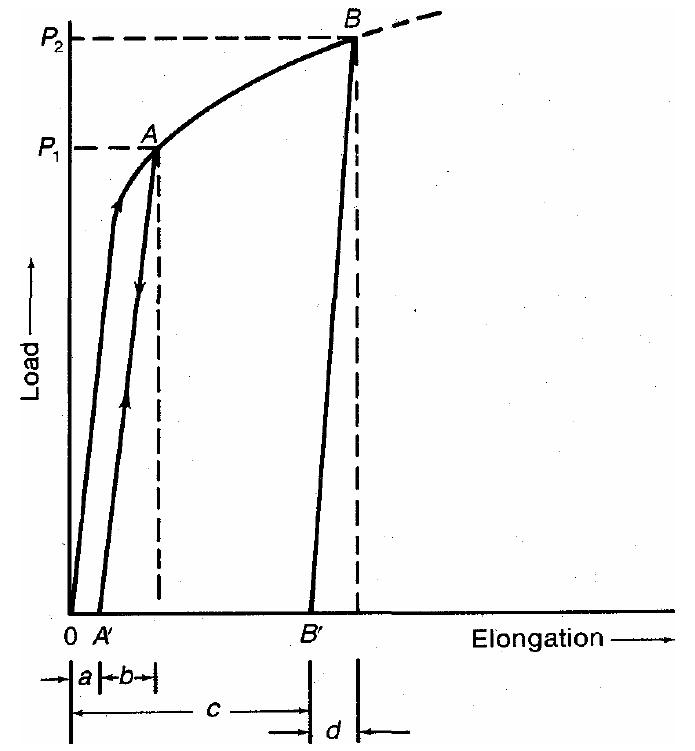
Figure 9. Schematic representation of un- stable fatigue crack growth. (Points A and B correspond to crack jumps.) Figure 10 compares fracture toughness characteristics of heat resistant and chrome— molybdenum steels under cyclic and dynamic loading. One can see a good correlation between K;. and Kjg. This suggests that fatigue fracture toughness characteristics of materials, similar in properties to those studied herein, can be judged from dynamic frac- ture toughness characteristics and vice versa. Based on the model formulated above, other possible cases of the relationship between fracture toughness characteristics under static, dynamic, and cyclic loading have been discussed in [26,31].

Figure 1. Description of device used by Leonardo daVinci for tensile tests on iron threads Scale effects were first mentioned by Leonardo da Vinci (1452-1519), who performed tensile tests in the following manner: a bucket was suspended from a beam on an iron wire (thread) the length of two “brasses” (3.248 m), Fig. 1. Fine sand flowing from a hopper filled this bucket through a narrow gap. When the total weight of sand plus the bucket overcame the load resistance of the iron thread, failure occurred and the bucket fell into a soil hole.

where C; is a constant, V is specimen volume, 58 corresponds to Weibull modulus value. Figure 2. Scale effect in tension, experiments of Richards [1], explained by Weibull theory

Figure 3. Scale effects in bending, experiments of Richards [1]

Table 1. Values of A,,and d.,computed by Malmberg from Morrison’s results

Figure 5. Scale effects in cylinder exposed to internal pressure, experiments by Cook [4] Cook [4] has studied scale effect on yield stress of pipe under internal pressure. He used three types of mild steels (designated A, B and C) and pipes of 6 different diameters. Ratio of external and internal diameter was kept constant and equal to 3. Assuming that there is no scale effect in tension he has plotted pressure at yield stress over tensile yield stress versus internal pipe diameter. Noticeable scale effect Cook has attributed to the existence of a critical layer, in which plasticity occurs when yield stress is overcome.

Figure 6. Scale effect on ductile fracture area. Experiments by Chechulin [5]

Figure 9. Scale effects on ductile fracture strain. Experiments by Carassou et al. [10]

The average value of the fracture stress is given by:

Figure 10. Scaling law by Carpinteri, based on defect distribution [12]. Experiments by Sabnis and Mirza [13]

3.1. Fractal character of fracture surfaces

Figure 14. Asymptotic scaling law of Bazant [16] for two asymptotic behaviours: plastic collapse and brittle fracture

5. CONSTRAINT TRANSFERABILITY PROBLEM IN FRACTURE TOUGHNESS

In addition to the size effect, the ligament size also influences fracture toughness. Figure 15 shows the influence of normalized notch length a/W (a is notch length and W is the width) on brittle to ductile transition, depending on temperature, as determined on precracked specimens of cast steel. For decreasing ligament size and increasing ratio a/W, the shift to higher temperatures is obvious [23]. Different master curves for nuclear waste container cast steel indicate clearly that transition temperature fp, is shifted to higher value when the ligament size increases. In the transition regime, fracture toughness increases with decreasing ligament size (Fig. 16).

Figure 16. Influence of ligament size on fracture toughness J, for nuclear waste container cast steel Figure17. Distribution of tensile opening stress along the distance for different ligament size

Figure 19 shows effect of geometry on failure distribution. where @= 2 for small scale yielding. This leads to:

Figure 20. Transferability curve for nuclear waste container cast steel, obtained by the Koppenhoefer method

Figure 21b. Scheme for determination of stress intensity factor for cracked three point bend specimen (notch of infinite acuity) Eq. (68)

Figure 22. Scaling law for a notch with opening angle ¥

Figure 27. The applications of Malmberg’s model [22] to Morrison results

Table 2. Summary of the described scaling laws

Figure 1. Increase of steel strength by irradiation The absorbed energy for crack propagation decreases with the increase of neutron fluence (Fig. 2). For example, the absorbed fracture energy for propagation of a crack to length 4mm in a non-irradiated specimen is 290 kJ/m*. After neutron irradiation to fluence 8.10° n/m’, the absorbed energy decreases to 220 kJ/m’ and after irradiation to fluence 5.107 n/m?, down to 165 kJ/m’.

Figure 2. Crack growth vs. absorbed energy for different neutron fluences

Figure 3. The effect of neutron irradiation of RPV metal on Charpy impact energy, transition temperature 7k, upper shelf energy, and the slope of transition zone

The morphology of fracture surfaces of Charpy specimens tested at upper shelf tem- perature, transition zone, and low shelf of Charpy curve is different (Fig. 4). At the upper shelf, the fracture surface is characterized by elements of ductile fracture. At the transi- tion temperature, a central zone of brittle fracture appears. The relative part of brittle fractured zone increases with decreasing temperature. The elements of ductile fracture disappear completely at low shelf temperature.

Figure 5. Container with two surveillance specimens

1.6 times. Figure 6. The IMS model of assembly for standard Surveillance program of WWER-1000 RPV located in the notch zone of the specimens and in the aluminium filler. The assembly was irradiated during one fuel cycle. The examination of temperature monitors showed that the irradiation temperature is lower than 302°C. The measurement data of neutron monitor activities proved that the accuracy of methods and programs used for neutron fluence estimation is better than 15 relative percents. It was established also that the neutron field on the standard assembly is highly inhomogeneous and the differ- ence between fluence value on different specimens from the same assembly row reaches 1 6 times.

where chloride ions cause cracking in stainless steels and aluminium alloys. Also, an environment causing SCC in one alloy may not cause it another one. In general, SCC is frequently observed in metal/environment combinations that result in the formation of a film on the metal surface. These films may be passivating layers, tarnish films, or dealloyed layers. In many cases these films reduce the rate of general or uniform corrosion. As a result SCC is of greatest concern in corrosion-resistant alloys exposed to ageressive aqueous environments (Fig. 2).

Stainless steel: fatigue crack initiated at the pit bottom

from left to right. If not stopped, this process wil go on until all metallic Zn is consumed. Basically this is what is happening when we use common zinc—metal hydride batteries, but also when we put a piece of zinc in acid and it dissolves in the solution by direct electrochemical corrosion. If we add reaction ( ) to reaction (2) we obtain reaction (3) (Fig. 4), which represents overall processes as a single chemical reaction of the redox type, but the mechanism of this reaction is, as documented previously, electrochemical in nature, and follows the laws of electrochemical kinetics. Therefore for good understand- ing and control of such processes the knowledge of electrochemical kinetics of all electro- chemical processes participating in corrosion processes is necessary.

use of reaction inhibitors (cathodic, anodic, or with double action) the corrosion rates can be considerably decreased and kept under control. But note that if thermodynamic data show corrosion processes are possible, corrosion cannot be stopped totally, because that would ask for inhibitor coverage of 100%, i.e. 9=1, which is impossible to be accom- plished in real systems. Figure 7 graphically presents Tafel lines for a hypothetical corrosion process with a single cathodic and anodic electrochemical reaction in which i, is the so-called exchange current Jensity, and is a main constituent of a Tafel constant a. When the numerical value of a is larger, 30 is the exchange current density, and that means that the Tafel line for the corresponding srocess will be shifted to the right in the diagram. The opposite happens if the exchange current Jensity is smaller.

point, and also the corrosion current density will be equal to the passive current i,. This is why many metals and alloys, when used in open systems (i.e. in contact with air) behave as passive. However, if the concentration of oxygen decreases for some reason, Tafel line will shift to the left (Fig. 8, right) and eventually reach the situation marked with 2. In this case, the intersection of polarization curves is in position 2 when corrosion current densi- ty is rather large. Hence, in order to be able to control corrosion rates, experimentally determined polarization (or corrosion) diagrams for each situation considered have to be known. Otherwise, one can make the situation even worse by mistake.

Figure 11. Anodic dissolution model of crack propagation [10]

Figure 10. Schematic representation of the pit growth mechanism [8]

In this reaction there are no electrons involved, therefore it is not electrochemical and does not depend on electrode potential. Therefore it can occur at any potential outside or inside a pit or a crack and supply hydrogen which, either escapes as bubbles from pits or cracks, or penetrates inside the metal in front of a crack tip making it brittle. This is supported by the fact presented in Fig. 2 (right), that even the presence of humidity in the atmosphere can cause susceptibility to SCC proportional to the value of relative humidity, i.e. the amount of capillary condensed water.

Figure 14. Scheme of typical results obtained by statically loaded smooth samples Tests on statically loaded smooth specimens are usually conducted at various fixed stress levels and time to failure of specimens in the environment is measured. The thresh- old stress R,, is determined when time to failure approaches infinity, Fig. 14. These experiments can be used to determine the maximum stress that can be applied in service without SCC failure, or to evaluate the influence of metallurgical and environmental changes on SCC [11].

obtained with modified techniques combined with microscopy [17]. For example, average stress corrosion crack growth rate can be determined from the depth of the largest crack measured on fracture surfaces of specimens, divided by the time of testing. In this procedure, SC crack is assumed to be initiated at the start of test, which is not always true. On the other hand, fracture mechanics implies that the structure already contains a crack or a crack-like flaw.

Evaluation of SCC by mec usually conducted with either a hanically precracked (fracture mechanics) specimens are constant applied load (Fig. 16a), or with fixed crack open- ing displacement COD, and the actual rate of crack propagation v = da/dt is measured (Fig. 16b). The magnitude of s force for crack propagation) is ress distribution at the crack tip (the mechanica driving quantified by the stress intensity factor K; (in the scope linear elastic fracture mechanics LEFM) for specific crack and loading geometry. As a result, the crack propagation ra e, logda/dt is plotted versus K;. These tests can be made such that Kj, increased with crack length (at constant or gradually rising applied load), decreases with increasing crack length (constant crack opening displacement CO approximately constant as the crack length changes (special tapered samples) [11]. D), or is

Many real problems in practice have been considered by applying the described nethods, and some of them are presented.

Table 1. Contribution of stresses and strains in the bogie for base/modified model 3.3. Failure anlysis of the radi-axial bearing of the rotary excavator C700S

Analyses of the stress field (Fig. 7) showed presence of 16% bending stress in the computation model with 6 DOF and 11% in the reduced model (based on verified good concept of designed geometry). Large strain and stress concentration is found around supports. Obtained results showed that the effect of improper welding was negligible.

Figure 6. Model of excavator bogie C700S

3.4. Failure analysis and reconstruction of the excavator platform ARS Kopel Table 4. Percentual portions of stresses and deformation energy

Operating wheel behaviour diagnostics, recovery and reconstruction of the excavator C700S O&K (Kolubara Metal Vreoci) are presented in Figs. 11-13, and in Table 5. The bogie-wheel is loaded in bending and torsion. The hollow shaft is of the greatest influence in the wheel behaviour.

3.6. Diagnosed behaviour of the rotary excavator cantilever (C700S)

Table 5. Percentual portions of stresses and deformation energy

Table 6. Percentual portions of potential and kinetic energy Table 8. Natural frequencies of considered variants (in Hz)

‘igure 18. Geometry and deformation of some model variants Table 7. Percentual distribution of the strain energy Ey

It is concluded that the implementation of new ties and the filling has been a reason- able solution in this case.

Figure 20. Models of deformed elements after tank car crash Three tank cars fell out of railway tracks in a crash. Elements of bogies and links between the cylinder and bed, and also the cylinder tank, have suffered local plastic deformation. The possibilities of future use of tank required some decision making and, accordingly, defining necessary operations for eliminating crash consequences. Models of deformed elements are presented in Fig. 20. The computational model is given in Fig. 21, and tank deformations and stress fields for critical elements are shown in Fig. 22.

The structure of the bogies consists of several parts as shown in Fig. 23.

Figure 28. Model for stress analysis of cracked pressure vessel 3.11. Recovery of the rotary furnace

Part of tube from the entrance to elliptical holes

Table 11. Stress in the critical zone [kN/cm’]

Stress field in the critical zone 0-40 kKN/cm? with step 5

Table 12. Computational results 3.13. Recovery of the fractured tooth (containing cracks) In order to define recovery procedures, if possible, two 3D models of 5 teeth (0 and 1 in Fig. 34) and the stress distribution have been analysed after gear-wheel failure in the Cement Factory mill, in Beocin. The behaviour of the fractured tooth part (170 mm in length) has been correlated to the entire tooth length of 650mm behaviour (without cracks). Note that the position of the stress lines is similar in both cases (the stress in model | is about 20% higher than in model 0, Table 13). So it is concluded that the frac- tured tooth can be in function. [i 7 EES kee. iy Se, ee, ae, Se, eee ee a oe a . ee, ee ee ee a i, ee . ns |

3.14. Recovery and reconstruction of excavator SchRs800 O&K structure

Table 14. Percentual distribution of stress and deformation energy

The substructure recovery and reconstruction are successfully accomplished hydro-cylinder) and cylinder at 15° from linear axis (thickness 15 mm); to add four verti cal locators between the cylinder, top and bottom plat 105° from hydro-cilinder linear axis connection; the exi nal vertical longitudinal plate, top and bottom platform p be transformed in the diaphragm with outlet (thickness 1 form plate, at 30°, 45°, 75° an sting location between the exte1 ate (at 90° from linear axis) is t 5 mm); in upper parts of the “IT column frame insert two triangle locators 80080015 mm (three plates — front and bac! triangle, and longitudinal cross plate); on joint locator point for upper and lower pilla section add locators with vertical sections, that is horizontal partial plate with its locator 15 mm thick.

Table 15. Diagnostical data for structural behaviour of excavator superstructure 3.15. The analysis of crack significance on rotary furnace ring

Figure 43. Stress and deformation, for crack lengths a, = 10.7 cm, a) = 15.72 cm, a3 = 26.8 cm

Table 16. Distribution of loading effects

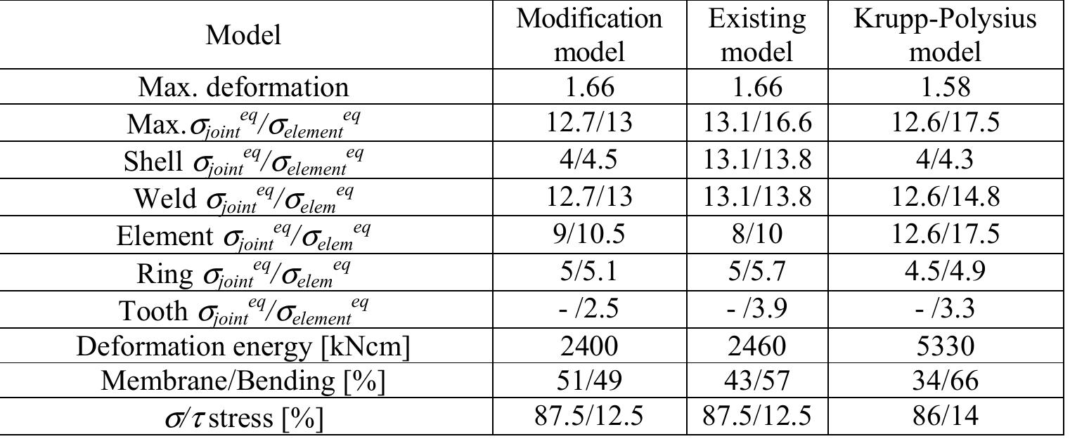
Table 17. Results of calculation (model, deformation [cm], stress [kN/em’], energy)

Figure 5. Geometry and dimensions of the fractured cross section (all measures in mm)

Figure 6. Distribution of membrane and bending stresses through thickness These values correspond to one half of the design nominal load (35 kN) for the fork. shown in Fig. 7, which is characterized by stress values 0; and oy at the front and back surfaces of the plate. Based on these data, a bending stress and a membrane stress com- ponents are determined as: oj, = 209 MPa; o;, = 2 MPa. These values correspond to one half of the design nominal load (35 kN) for the fork.

Fracture mechanics analysis makes a difference between the through crack, embedded crack, and surface crack. Real crack shapes are idealized by substitute geometries such as rectangles, ellipses, and semi-ellipses. The idealization has to been done such that crack tip loading will be overestimated. Sometimes a crack or cluster of cracks have to be re- characterized if they interfere one with each other, or with a free surface. Real, irregular cracks are modelled by “ideal” straight, elliptical, or semi-elliptical cracks with dimen- sions defined by their envelope rectangles, as shown in Fig. 9. Most important is that the idealized flaws yield conservative results of FE analyses, as compared to the original crack. A cluster of multiple flaws may interact. If multiple cracks are located close to each other in the same cross section, they will be more severe than single cracks. This is taken into account by interaction criteria. If the spacing between single cracks is less than a certain value they have to be replaced by a larger crack, like if they have already coincided, as shown in Fig. 10. In a similar way the interaction effects between cracks on free surfaces are treated.

Usually, the crack plane is assumed to be perpendicular to the larger of the two principle stresses. In some cases, however, a real crack will not grow within this plane because of mechanical reasons, i.e. both principal stresses are of a magnitude of the same order, or because of the material heterogeneity. In such cases a more complicated mixed- mode analysis has to be carried out. In the present case the situation is quite simple because the maximum principle stress direction is identical to the axis of the fork. In the flow chart in Fig. 3 the crack dimensions are introduced as input data. Actually, this refers to 9 default crack size which is then varied iteratively Tn each iteration sten

Figure 12. Definition of strength mismatched configuration Mismatch of strength means that in the welded joint, the base plate and the weld metal are of different strength, with the consequence of local strain concentrations within the weaker area if the yield strength of weld metal differs more than 10% from that of the base metal; if this difference is bellow 10%, the use of SINTAP procedure for homoge- neous material (base plate) is recommended. The weld metal is commonly produced with yield strength, Oy, greater than that of the base plate, yg. In Fig. 12b this case is desig- nated as OverMatching (OM) with the mis-match factor M,

Table 1. Mechanical properties obtained by tensile test and Charpy impact toughness values

Figure 15. Engineering stress-strain curves of the fork material

where Fy is the yield load of the cracked configuration.

Figure 17. Failure assessment based on the CDF philosophy (The function f(L,) is identical for the FAD and CDF routes)

Figure 18. Test setup for determination of critical crack tip opening displacement Table 2. Charpy energy of the fork material at different temperatures

The fork of a forklift is an example for using “Default” level, level “1” and level “3”. In Figs. 20 and 21 the CDF and FAD analyses are demonstrated for a crack size of 2c = 45.5 mm. This length corresponds to real crack length measured on the fractured surface of fork, as shown in Fig. 22. It is shown that the higher analysis levels yield less conservative results. The Default Level which uses fracture toughness values estimated from Charpy energy gives much lower critical loads than the higher levels.

Figure 21. FAD analysis of the fork assuming a crack width of 2c = 45.5 mm. The predicted failure loads are identical to those obtained by the CDF analysis in Fig. 20

Figure 22. Real crack length measurement of the fractured fork

Figure 1. Conversion of the contour integral into an Equivalent Domain Integral method (EDI)

2. THE ESTIMATION OF FATIGUE LIFE Unstable crack propagation occurs when one of the stress intensity factors Ky (@= I,JI,II1) is equal or greater than the experimentally determined material property K,. The estimation of fatigue life can be updated for each crack extension. The crack growth equation provides a relation between the crack increment Aa and the increment in the number of load cycles AN. In case of cyclically loaded structures, the number of load cycles equivalent to the crack increment can be determined by a numerical integration of the governing crack growth equation [11]. Te Dad ee Tiascex: Sx or wile Te: lewsk esnes i tieaw sven waenolal &® neanle wenscsth. awante Ane nedndiing be

Table 1. Comparison of results In order to present robustness of the J-EDI procedure, built into the PAK software, the above example was used with different radii rz of the integration domain and the results are shown in Table 2. Radius rz varied from 0.5% a to 90% a, where a denotes crack length. It can be concluded from Table 2 that results are insensitive to the choice of the J— integral domain integration radius.

Table 2. Values of the factor Kj for different integration domain radii

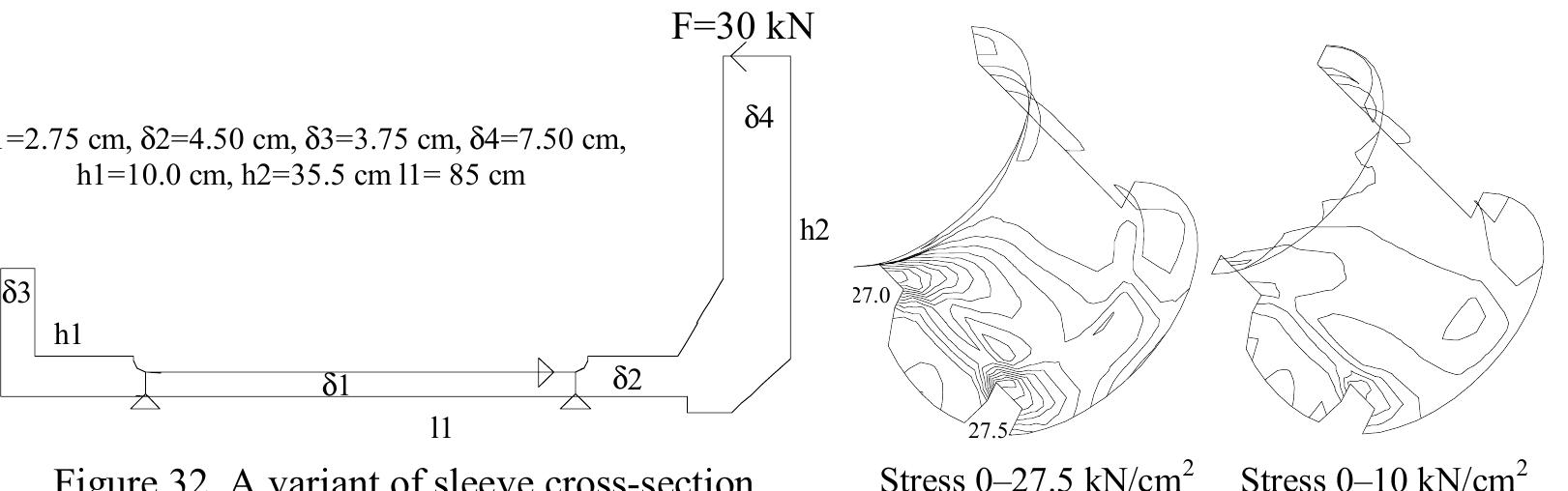
In this example [14], a 3-D analysis of the turbine housing is carried out. Using the original design documentation, the 3-D geometrical model of the turbine is generated. In this 3-D object, cracks with different lengths (90-375 mm) and depth (20-40 mm) are assumed and modelled. Calculations are performed to investigate the influence of crack length and depth on the value of maximum effective stress, as well as on the value of stress intensity factor.

Figure 8. Relationship between stress intensity factor Kj and crack length Figure 7. Effective stress field for crack length 30 mm

Figure 11. Field of the effective stress in the vicinity of the crack (375x30)

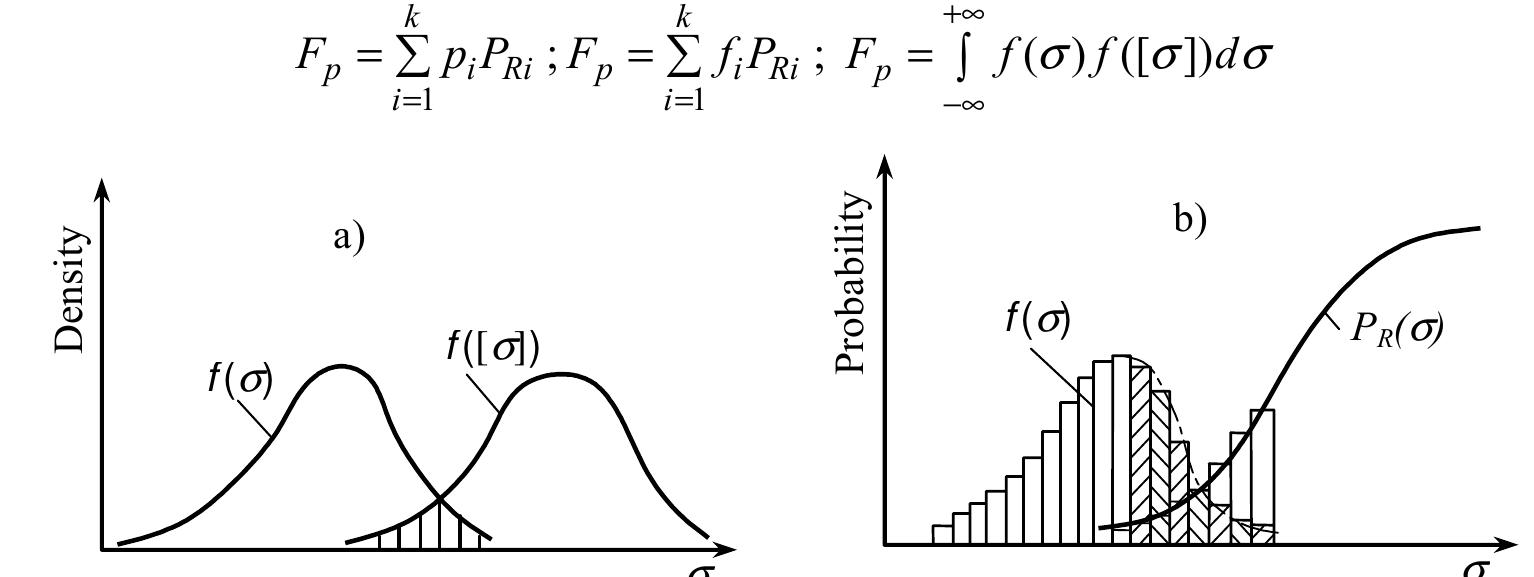
Figure |. Relation between service stress distribution f(0) and critical stress distribution f([o]) in safety factor determination nor the work stresses are determinant values. The determinant values are stochastic values which dissipate by rule within a wide range (Fig. 1). The safety factor is the ratio of the mean (most probable) value of critical stress and the highest work stress, which can be expected in the work process. There is also a possibility for the occurrence of circum- stances which cannot be foreseen, thus work stress can be somewhat greater, but this is not likely. The machine part has absolutely been used, and the safety in work satisfied, if the safety factor is such that the highest possible value of work stress is lower than the minimal possible value of critical stress. This condition has been satisfied if the dissipa- tion presented in Fig. 1 (curve 1) is covered by the value of the safety factor. This value is S=1.25...2.5. Lower limits may be used when data about the critical and work stresses are well known and reliable.

HUT OL ALIO WOU SU SD 1d URLOLITIIVU Uli UI Udols Ul KUUWiIt UlsUUUUOLE UL UI WULKIIIE Ali critical stresses and for the chosen value of reliability. The elementary reliability relates to the possibility of occurrence of certain kinds o . 5 j occurrence fracture to occur due to fatigue, it is necessary that stress occurs in the machine part an cated condi hat the pos he density . efects, i.e. failures. The unreliability, F,= 1—R, is a complex probability of th probability of C service stress, and of the probability of failure at that stress. Fo sibility of fatigue (fracture) exists at that stress. Fracture occurs if both indi ions are satisfied, i.e. the probability represents the integral of the product o of these probabilities and is proportional to the overlapping area in Fig. 2¢ The integration is obtained numerically and turns into the sum of the product of th ensity of s ress probability f; and failure probability Pr; which represents the cumulativ (integral) probability of critical stress. If the number of different service stresses i is small, the probability density f; turns into the statistical weight p;. It can be determined as the ratio of stress fluctuation o; cycles number in the length of service ms; and the total number of s ress cycles in the length of service Ny, i.e. aS p;= Ny/ny. If a machine part is exposed to a fluctuating stress of constant amplitude, the statistic weight, 1.e. the possibility of t he occurrence of such stress is p(G) = ny/ny = 1, thus the unreliability is equal to failure probability Pe(o). If a machine part is exposed to stresses of different amplitudes (Fig. 3), the Di = Ns/ny (Ny = Yns;). In that proportion, the failure probabi the unreliability F,, (Fig. 2b and Fig. 3). The unreliability is e of statistic weight and failure probability for each one of the s statistical weight of each is ities Pr; have an impact on qual to the sum of products ress values.

Figure 3. The relation of failure probability and work stress in the range of infinite life strength

The presented procedure enables cumulative probability F,, to be obtained for variable stress amplitude, based on the function of distribution of failure probability Pp; for constant stress amplitude. This approach is acceptable for most defects of which it is necessary to fulfil two conditions: that the cause of defect exists and that this cause is capable of producing the defect. This means at the same time that functions presented in he shape of proba critical stresses. T opposite. In order critical stresses, it Fig. 2 are mutually independent. In fractures due from fatigue, these two curves are no independent. The position of the function of failure probability distribution Pr depends on he density maximum centre is towards lower stress values, that is a light exploitation regime. For light regimes the function Pr moves towards the zone of greater values of ions, and unreliability F,, is reduced. In case of heavy exploitation regimes, the process is bility density f(o) function. If the function f(c) is asymmetrical so tha he curves f(a) and Pr become mutually distant for such work condi- o take into consideration relation between distributions of service and is necessary to introduce into consideration the failure probability for service fatigue strength. Figure 4 shows the function and the range of distribution of the failure probability for the service fatigue strength. Figure 4. The relation of stress distribution (0) and failure probability Pp for service fatigue strength

Figure 5 shows the possible analogous random function of stress fluctuation with marked values of change, i.e. stress change ranges 0, = 20,, where O, is the stress ampli- tude. The mean values o,, around which stress fluctuates, are also variable. It is necessary to make a selection of values of the changes and their mean values, classify them into classes and determine the number of occurrences of each of the values of changes. If the analogous (uninterrupted) time function is digitalized, it transforms into a set of numeri- cal values in small time intervals At, as presented in Fig. 5a. The program for processing digital values compares each one of them with the previous one and determines the values of neighbouring extremes — minimum and maximum, and calculates the spans o;;= Omaxi — Omini: The span is calculated only at the increase of stress so that the cycles are not doubled. The calculated spans can be classified by their value and by mean stress values. For the purpose of simplification, further analysis relates only to spans. Figure 5b shows that the calculated values of the spans are classified in certain classes — fields of equal value. For example, the first class, for i= 1, would include all spans o,; = 0...20 N/mm’, and the second for i = 2 would include spans oj = 20...40 N/mm”, and the third for i = 3, 03 = 40...60 N/mm’ ete.

Figure 7 shows the coordinate system with uniform scale on the coordinates X and Y (upper and right scale). Starting from expressions for X= Ino, and Y= InlIn{I/[l — F(o,)]} and from this uniform scale, values have been calculated for o, and for F(o,), the values of which are given on the lower and left scale. This is how the Weibull’s coordinate system is obtained. Experimental (empirical) values of cumulative probability F(o,) are entered for each class of stress amplitudes o,. A series of points is obtained which follow closely the straight line. After entering, this set of points is approximated by a straight line. Coordinates X and Y enable determination of parameters in the equation of the straight line, a and 6, and t After approximating experimental points by a straight line, the parameter 77 expressed in the stress units is read in the intersection of the straight line with the X axis, i.e. that is the stress value for the probabi thus in expression F(0;,) the ratio o;,/77 is a dimensionless value. Parameter G= 1.3 is the part on the Y axis for AX = The greatest stress fluctuations have the greatest effect on fatigue of the material. The hereby also the parameters of Weibull’s distribution, 7 and 2. ity F(0,) = 0.632. Dimensions of parameter 77 are same as O;, and represents a dimensionless value. where the independent variable x is substituted by the stress amplitude o,. The parameters of this distribution are 7 and f, which may be determined in the simplest way by graphi- cal method. It is necessary to transform Weibull’s function into the form of a straight line for this purpose. This is achieved by double logarithm of the transformed form of Weibull’s function

Figure 7. Parameters of Weibull’s function determination for stress amplitude distribution units on the logarithmic axis with the scale from 100 to 106 stress cycles (Fig. 8). With this transformation the cumulative function F(o;,) has been translated into the logarithmic form, where the range of large stress amplitudes has been spread out onto about 2/3 of the horizontal axis, and the field of small and medium stress amplitudes has been compressed onto 1/3.

The continuous shape of the logarithmic curve is not suitable for use in calculations or for endurance testing. The step-like shape is more suitable for this purpose. The optimal number of steps (stress levels) is eight. The division is formed by forming more steps in the range of greater values of stress amplitudes (differences in stress levels are smaller), and in the range of smaller amplitudes there are less steps with greater differences in level. After the division it is possible to create a tabular form, i.e. a table filled up with values which are read from the graphical presentation (Fig. 8).

Table 1. Presentation of the stress spectrum in Fig. 8 The Stress Spectrum is an ordered set of stress amp the participation of each of the stress amplitudes o; in ical (ordered) presentation of random stress to be defined in the random process and res completed. The stress spectrum is determined by the value n,, the relative variable x;, and stress 0). The number of stress levels may a by statistical processing of empirica random function, as has been shown above, or starting from the itudes F(o,). Besides this, the stress spectrum can is a statis behaviour the larges less than eight. It can be obtained growing function of stress amp obtained by combining the deterministic and length the machine system may operate wi (stresses) may be calculated and it is also cycles of each one of them. By joining the and number of cycles, a set of blocks is ob number of cycles to n, and blocks to Anyj;, need not satisfy the above given conditions itudes of the value n, which shows he selected number of cycles ny. It fluctuation, it enables a pattern in pective calculations and tests to be be greater but also significantly data obtained from known cumulative be he course of service sO statistical approach. In t h different loads (stresses). The load values possible to estimate the possible number of blocks of stress cycles defined by the value ained. By proportional reduction of the total a stress spectrum is obtained. This spectrum by all its features, but it may be used both for testing and for calculations, and also for es imates of the service regime. The mentioned possibilities of stress spectrum formation do not give the same degree of precision. The choice is made depending on the aims and possibilities of realization. NRA. .4.°% 2 2 . PRaP = ._.. . ££. BS. | aac: fe oe - £ ». gt ge = @. = i.

Figure 9. Characteristic representatives of light (/), medium (m) and heavy (/) exploitation regimes decreasing presence of small amplitudes. By further increase of the severity of the exploitation regime all amplitudes become equal to the highest. That is the regime with a constant stress amplitude (x,, = 1). If Weibull’s distribution function of stress amplitude F(0,) is known, the appraisal of the severity of the exploitation regime may be made if the amplitude with the highest occurrence frequency is determined. Another derivative of the function F(o;,) equated to zero determines the extreme of the function maximum /(0,), where

The failure probability is a cumulative probability that a machine part will fail under a certain stress by a certain stress cycle number. This is also the probability that at a certain stress cycle number, failures will occur at certain stresses. The failure probability is calcu- lated on the basis of statistical processing of the testing results. That is the ratio of the number of failed test samples (parts) under certain conditions and the number of tested parts under such conditions. It is necessary to choose for testing, the stress values to which the test samples, i.e. parts are to be exposed, then the number of pieces which are to be tested, and the manner of achieving (simulating) the stress fluctuation. The number of pieces (test samples or parts) zy to be tested on each one of the chosen stress levels should be sufficiently big so that, based on the sufficiently big set, it would be possible to deduce statistical conclusions. A set greater than zx = 20 test samples or parts is consid- ered as sufficiently big. This testing work takes a lot of time with significant energy consumption, and the tested parts are not for further use. It is therefore endeavoured to reduce as much as possible the number of pieces to be tested. The smallest number of pieces which still makes possible the deduction of statistical conclusions is zy = 8. For these small samples the failure probability is not defined as the ratio of the number of failed z; and tested pieces zs, Le. aS Pr=z,/zs, but as by some of the approximate expressions 7 z.—-05 | z.—(0).33

The manner of achieving (simulating) the fluctuating stress is another of the signifi- cant issues which must be resolved at the performance of research. Figure 11 shows some of the possibilities of achieving the fluctuating stress with constant amplitude. Rotating test samples exposed to rotating bending (Fig. 11a) are simply loaded with calibrated weights through roller bearings. Due to the rotation of test samples, reverse stress changes

Figure 14. Definition of the parameters of Weibull’s distribution for the failure probability in the range of infinite—life strength

| we aisle caine ON with the use of respective parameters 7 and £2. In this way points are determined for stres: evels Oy, and Oy? and for the number of stress cycles Npy. The calculated coordinate have been entered into the coordinate system with logarithmic axes, Fig. 15. By joinins he points with the same probability Pr, border curves are obtained Pr = 0.1, Pr= 0.9 a well as the middle line for Pr = 0.5. The failure probability distributions have been pre sented on stress levels oy, = 973 N/mm7, dy = 810 N/mm” and for Npy = 5:10°. Based ot border lines, it is possible to define distributions for any stress Oy and for any number o stress cycles N. The middle line in the dissipation field, for failure probability Pr = 0.5 represents Wohler’s S—N curve. It is defined by three parameters Op (Ojim), Np and m. The coordi- nates of breaking point are Op = Ojim = 748 N/mm? and Np = 2.5-10° and are defined by reading from the diagram. The exponent by which the inclination of W6hler’s curve is defined is obtained on the basis of coordinates of points on this line, i.e.

The service fatigue strength Op follows the curve in the double logarithmic coordina system (Fig. 16a). By approximating this slightly curved line with a broken up straig ine, a line is obtained with two breaking points, the coordinates of which are presented he figure as equations of the parts of these lines. The coordinates of the breaking poi Oro, Nro and the exponent g are parameters of the service fatigue strength curve. TI position of the curve in the coordinate system depends on the weight of the work regim In case of the light one (/), the curve is shifted to the right, i.e. towards the range | extremely high numbers of cycles up to fracture Ne. With an increase of the heaviness | he regime, the service fatigue strength curve approaches the Wohler’s (w).

The simulations are materialized by starting from some stress level from the spectrum block) centre. Upon completion of the simulation of stress level oy, for example, with the aumber of cycles ANga, a transition is made onto a higher stress level 03 and so on up to 0, and then from the biggest stress level towards smaller ones as presented in Fig. 17. If lock Nz is smaller, it will be repeated several times up to fracturing, i.e. the number of epetitions is y = Ne/Nz. Better mixing of big and small stress amplitudes suits the greater aumber of repetitions. Too big number of repetitions of blocks imposes the need for the inacceptable big number of stress level change in the course of the testing process. This oroblem may be resolved by electronic, i.e. program management of stress level changes. For the determination of failure probability for service fatigue strength, test results are required for three stress levels Op, i.e. Oj. Two levels are required for the determination of the direction of the lower part on the service fatigue strength curve. The upper part of this broken straight line is parallel with the line of the basic (Wéhler’s) strength. Testing is necessary for one stress level for the purpose of determination of the position (distance) of this part from the line of basic strength. The highest stress level op’ is chosen in such a manner that all stress levels in the stress spectrum are greater than the infinite life strength. The lowest stress level in the spectrum must thereby be significantly above the infinite life strength, so that the greatest stress in the spectrum oO,’ is in the zone of the

Figure 19. Distribution functions of the failure probability for service fatigue strength

Figure 2. Different zones formed in the heat-affected-zone (left) and in the weld metal (right) of a multi-pass welded joint, therefore having different properties

Figure 5. Thermal conditions at fusion line simulated for single-(top) and double-pass welding (bottom) HV max = 802% %C +305

Figure 6. Continuous-cooling-transformation (CCT) diagrams valid for CGHAZ of two steels: HSLA steel Nionicral 70 (left) and StE 355 Ti, fine-grained steel, microalloyed with Ti (right) will never exist if 7,2 = 780°C. Bainite in both double-cycle HAZs is formed at shorter Atgs than in CGHAZ (Fig. 6—left). Smaller portion of ferrite is already present at much higher cooling rates than in the case of CGHAZ. All this is reflected in Vickers hardness of formed HAZs (numbers in circles). The obtained CCT diagram that corresponds to T,2 = 780°C is valid only for the retransformed part of the former CGHAZ. The rest of microstructure is tempered former single cycle CGHAZ.

Figure 7. Continuous-cooling- transformation (CCT) diagrams valid for different double-cycle heat-affected-subzones close to fusion line of HSLA steel Nionicral 70. Due to differences in peak temperatures T,,. the microstructures are not the same.

Figure 9. Charpy specimen machined from the sample with simulated microstructure of the CGHAZ (left), and its S-curve (right)

Figure 8. Hardness HB (left) and V notch Charpy impact toughness at —40°C (right) for specimens, simulated at different temperatures T,, meaning across the whole width of the HAZ

Figure 10. Impact toughness against Afg/s for a single cycle CGHAZ (left), and against 7, for HSLA structural steel Nionicral 70 (right). Double-cycle HAZ was previously CGHAZ.

Figure 11. Experimental determination of mechanical and rheological properties of material with the simulated microstructure

Figure 13. Logarithmic dependence true stress—true strain for determination of strength coefficient A and plastic strain exponent n

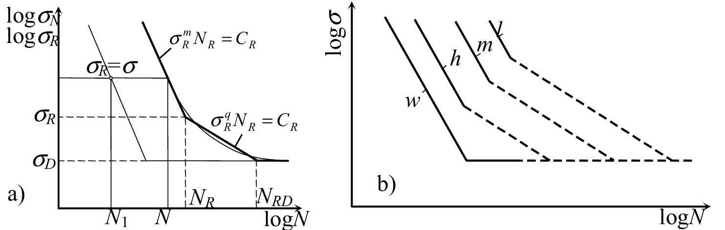
The result of final evaluation is shown in Figs. 20 and 21 [21].

The Kg values of both ICCGHAZs agree fairly well across the whole temperature range of CTOD testing (40 to 0°C). The agreement between Keg values of both CGHAZs is acceptable only at —40°C, but not at higher temperatures. However, values in Figs. 20 and 21, which are derived from diagrams recorded by CTOD testing, are in general, in spite of adaptation, less optimistic than the others. The reason is the character- istic geometry of both fracture toughness specimens.

Figure 22. The appropriate specimen for measurement of fatigue crack propagation rate (left), and for the endurance limit (right) in HAZ Two types of specimens were used to determine some fatigue properties of simulated microstructure found in HAZ of welded joints. They are shown in Fig. 22. Simulated microstructure exists at the mid-length of the samples. The appropriate shape of specimens and the type of loading must be taken into consideration. Strength of HAZ can be higher than the strength of the base metal. In general, fatigue properties increase with strength. Relevant fatigue properties will be available only if the fatigue process takes place in the mid-length of the specimen.

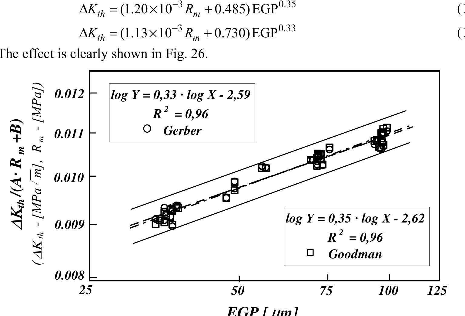
Figure 23. The fatigue crack propagation rate (left), and three courses of the endurance limit Two types of surface defects were considered: single Vickers indentations and series of Vickers indentations. The size of each indentation was either d=110um or d= 220 um. Both kinds of artificial defects are schematically presented in Fig. 24—left [27,28]. Equivalent geometrical parameters (EGP) of these artificial defects were calcu- lated. Defect size and stress gradient were also taken into account [13]. They are shown in Fig. 24-richt.

Figure 25. The fatigue strength for twelve different structures in HAZ The effect is clearly shown in Fig. 26.

Figure 26. The threshold stress intensity factor range normalised with the strength of the material

Fracture mechanics has brought significant changes in engineering prac example to illustrate this statement, the problem with the Alaska pipeline and ice. As an application of the fracture-safe principle in design may be mentioned. In case of the pipeline from Alaska to the rest of the USA, the fracture mechanics criteria were adopted traditional standards on admissible defects in a welded joint [12]. Namely, instead of when non- destructive testing revealed a large number of defects in round welded joints which, according to the then effective standards, should have been repaired, the ques nomic justification, i.e. necessity of repair, arose. Therefore, the institution ion of eco- in charge,

SPEEA ACCA, STEEN: SDINSDE OMS NON MOTTE In order to be able to analyze a crack, one should present it in some of the forms for which analytical solutions do exist. Cracks are divided into passing-through and partially- yassing, the latter being divided into surface and hidden types, Fig. 4. If there are more sracks, the increase of stress intensity factor should be taken into account, while at very ‘lose distances the cracks join into a single one, Fig. 5. The procedure of crack analysis ilso includes its projection in the plane normal to the direction of main stress, and the lescription of a rectangle, the dimensions of which are taken as its basic dimensions.

3.1. Pressure vessels at hydroelectric power plant ‘Bajina BaSta’ not only about the stress distribution, but also about the division of loading into primary and secondary loading. Primary stresses mainly occur due to exterior loading and moments, while secondary stresses are most frequently the result of effects of non- uniform heating and cooling, e.g. welding—induced stresses that are localized and self— balancing. Unlike secondary ones, primary stresses may lead to yield fracture, if suffi- ciently strong. Secondary stresses contribute to fracture, if tensile, with sufficiently high values and close to a crack.

3.1.1. The analysis of critical defects using the methods of fracture mechanics The defects marked as ‘critical’ were analyzed using methods of fracture mechanics, by applying conservative approach. Therefore, all three were considered as cracks: defects No.970-64 and 978-14 as surface cracks (partially passing through the thickness, while defect No.971-57 was considered a line crack (passing through the entire thick- ness). In this way an extremely conservative assessment was adopted for defect 971-57, in order to check the behaviour of the vessel, even in such a case. id have been eliminated by grinding, with small reduction of thickness at the grinding , which had no significant influence on vessel safety [22]. Jessel No.976 had 5 defects marked as unacceptable, according to Report No.6/98 of a Institute, out of which defects from Photos No.24 and No.38 were again, ultrasoni- y inspected. Based on additional ultrasonic inspection, it was concluded that two slags 1 Photo No.976-24 were not connected, and that the defect from Photo No.976-38 in fact offset or mismatch, i.e. shape defect (507). Having this in mind, as well as the and location of defects found in vessel No.976, it was concluded that all five defects essel No.976 were less dangerous than those marked “critical” in vessels 970 and 971. Jessel No.978 had 5 defects marked as unacceptable, out of which the defect from to No.35 was additionally ultrasonically inspected. Additional ultrasonic inspection ved that dimensions of this defect were not ‘critical’; but incomplete penetration 402, 25 mm long, from Photo No.978-14 was chosen as one of three critical defects, ough additional ultrasonic inspection failed to register it. The width of this defect, the ie of 2 mm was adopted that, according to the documentation of vessel No.978, corre- ided to the predicted size of the weld metal root, and at the same time was the upper itivity limit for ultrasonic examination. as ~~ 4 oe ee ee ee

Figure 10. Cylindrical part scheme in which crack No.971-57 is analyzed cylindrical part of the vessel, since in the torus area adjacent to the cylindrical part the stress is pressure, and not dangerous for crack growth. Thus, non-symmetry in the problem, caused by the location of crack is ignored, and same as in the previous case. If the sum of longitudinal stress, caused by internal pressure (‘boiler formula’), and trans- versal residual stress in the centre of the seam is assumed to be the remote stress, than the following is obtained for stress intensity factor: fn \ LAO nN7An \

Figure 11. Failure analysis diagram for damaged vessels

During the period from 1995 to 1996 the pipeline was subjected to inspection a few times, using various methods of non-destructive testing which, among others, revealed longitudinal defects (cracks) in longitudinal welded joints II and III, where bent sheet pieces were inserted on the part of increased thickness (50 mm), Fig. 12a. Having in mind the dimensions of cracks, the crack in the joint III, Fig. 12b, was taken for analysis, as more dangerous.

The calculation of stress state using the finite element method (FEM) is made based on the model shown in Fig. 14 (a quarter of inserted pipe). The results of analysis pre- sented in Tab. 1 show that the collar decreases stresses from 144 MPa to 80 MPa, in the region of pipe parts 250 mm away from the middle of the collar, which corresponds to the location of joints with cracks. However, even with so reduced operating stress, the corre- sponding point in FAD drops into an unsafe region, as the value for S, modifies to 0.7, while the value of K, remains unmodified (0.99). However, one should have in mind that Considering the conservative approach in the analysis of critical failures, crack III is assumed to have 30 mm depth over the entire observed length. In this case the problem should be considered in the section oriented transversally to the longitudinal direction of the vessel, where the curvature effect is ignored and quite justifiable for 50 mm thickness and 2400 mm diameter. The analysis becomes two-dimensional (plain strain) and the problem is considered as a plate under tension with an edge crack. If the remote stress is assumed to be the sum of circumferential stress induced by internal pressure (‘boiler for- mula’) and the residual stress in the weld centre, the stress intensity factor is as follows: we a Se: i a ae ~~

Table 4. Stresses at characteristic points along the bifurcation axis — with upper plate on the collar

Key takeaways
AI

Fracture mechanics provides critical insights into the integrity of materials and structures under stress.
Neutron irradiation significantly embrittles reactor pressure vessel (RPV) materials, increasing transition temperatures and decreasing toughness.
Stress corrosion cracking (SCC) and corrosion fatigue are major failure mechanisms influenced by environmental and mechanical factors.
Fracture mechanics standards, such as ASTM E399, guide the assessment of material toughness and crack behavior.
The SINTAP procedure offers a systematic approach for flaw assessment in engineering materials, enhancing safety and reliability.

References (390)

Kanninen, M.F., Advanced fracture mechanics, Oxford Engineering Science Series, Oxford University Press. (1985)
Griffith, A.A, The Phenomena of Rupture and Flow in Solids, Philosophical Transactions of the Royal Society of London, A221, pp. 163-197, (1921); and The Theory of Rupture, Pro- ceedings of the First International Conference of Applied Mechanics, Delft. (1924)
Griffith, A.A, The Theory of Rupture, Proceedings of the First International Conference of Applied Mechanics, Delft, pp. 55-63, Biezeno and Burgers ed. Waltman. (1925)
Inglis, C.E., Stresses in a Plate Due to the Presence of Cracks and Sharp Corners, Transac- tions of the Institute of Naval Architects, 55, pp. 219-241. (1913)
Bueckner, H.F., The Propagation of Cracks and the Energy of Elastic Deformation, Transac- tions of the American Society of Mechanical Engineers, 80, pp. 1225-1230. (1958)
Erdogan, F., Stress Intensity Factors, Journal of Applied Mechanics, 50, pp. 992-1002. (1983)
Sneddon, I.N., The Distribution of Stress in the Neighborhood of a Crack in an Elastic Solid, Proceedings of the Royal Society of London, A187, pp. 229-260. (1946)
Westergaard, H.M., Bearing Pressures and Cracks, Transactions of the American Society of Mechanical Engineers, 61, pp. A49-A53. (1939)
Irwin, G.R., Analysis of Stresses and Strains Near the End of a Crack Traversing a Plate, Jour- nal of Applied Mechanics, 24, pp. 361-364. (1957)
Sih, G.C., Paris, P.C., and Erdogan, F., Crack Tip Stress-Intensity Factors for Plane Extension and Plate Bending Problems, Journal of Applied Mechanics, 29, pp. 306-312. (1962)
Sih, G.C., Paris, P.C., and Irwin, G.R., On Cracks in Rectilinearly Anisotropic Bodies, Interna- tional Journal of Fracture Mechanics, 1, pp. 189-203. (1965)
Elliott, H.A., An Analysis of the Conditions for Rupture Due to Griffith Cracks, Proceedings of the Physical Society, 59, pp. 208-223. (1947)
Cribb, J.L., and Tomkins, B., On the Nature of the Stress at the Tip of a Perfectly Brittle Crack, Journal of the Mechanics and Physics of Solid, 15, pp. 135-140. (1967)
Goodier, J.N., Mathematical Theory of Equilibrium Cracks, Fracture, H. Liebowitz (ed.), Vol. II, Academic, New York, pp. 1-66. (1968)
Rice, J.R., A Path Independent Integral and the Approximate Analysis of Strain Concentration by Notches and Cracks, Journal of Applied Mechanics, 35, pp. 379-386. (1968)
Gehlen, P.C., and Kanninen, M.F., An Atomic Model for Cleavage Crack Propagation in Alpha Iron, Inelastic Behavior of Solids, M.F. Kanninen et al.(ed.), McGraw-Hill, New York, pp. 587-603. (1970)
Weiner, J.H., and Pear, M., Crack and Dislocation Propagation in an Idealized Crystal Model, Journal of Applied Physics, 46, pp. 2398-2405. (1975)
Ashurst, W.T., and Hoover, W.G., Microscopic Fracture Studies in the Two-dimensional Triangular Lattice, Physical Review B, 14, pp. 1465-1473. (1976)
Markworth, J.A., Kahn, L.R., Gehlen, P.C., and Hahn, G.T., Atomistic Computer Simulation of Effects of Hydrogen and Helium on Crack Propagation in BCC Iron, Res. Mechanica, 2, pp. 141-162. (1981)
Irwin, G.R, Kies, J.A., and Smith, H.L., Fracture strengths relative to onset and arrest of crack propagation, Proceed. of the American Society for Testing Materials, 58, pp. 640-657. (1958)
Wells, A.A., Applications of fracture mechanics at and beyond general yielding, British Weld- ing Journal, 10, pp. 563-570. (1963)
Dugdale, D.S., Yielding of steel sheets containing slits, Journal of the Mechanics and Physics of Solids, 8, pp. 100-108. (1960)
Muskhelisvili, N.I., Some Basic Problems in the Mathematical Theory of Elasticity, Nordhoff, the Netherlands. (1954)
Barenblatt, G.I., The Mathematical Theory of Equilibrium of Crack in Brittle Fracture, Advan- ces in Applied Mechanics, 7, pp. 55-129. (1962)
Eshelby, J.D., The Continuum Theory of Lattice Defects, Solid State Physics, Vol.3, Academic Press. (1956)
Rice, J.R., The Mechanics of Crack Tip Deformation and Extension by Fatigue, Fatigue Crack Growth, ASTM Spec. Tech. Publ., p.415. (1967)
Williams, M.L., On the Stress Distribution at the Base of a Stationary Crack, Journal of Applied Mechanics, Vol. 24, No.1, Trans. ASME, Vol. 79, Mar. 1957, pp. 109-114.
Irwin, G.R., Fracture Mechanics, Structural Mechanics (Proceeding of first Naval Sympo- sium), Pergamon Press. (1960)
Rice, J.R., Mathematical Analysis in the Mechanics of Fracture, Treatise on Fracture, Vol.2, ed. Liebowitz, H., Academic Press.
Hutchinson, J.W., Fundamentals of the Phenomenological Theory of Nonlinear Fracture Mechanics, Journal of Applied Mechanics, 50, pp. 1042-1051. (1983)
Sanders, J.L., On the Griffith -Irwin Fracture Theory, Journal of Applied Mechanics, Vol.27, No.2, Trans. ASME, Vol. 82, Series E, June 1960, pp. 352-352.
Thomas, A.G., Rupture of Rubber, II, The Strain Concentration at an Incision, Journal of Polymer Science, Vol. 18. (1955)
Rice, J.R., Drucker, D.C., Energy Changes in Stressed Bodies Due to Void and Crack Growth, International Journal of Fracture Mechanics, Vol.3, No.1. (1967)
Bowie, O.L., Neal, D.M., The Effective Crack Length of an Edge Notch in a Semi-Infinite Sheet Under Tension, International Journal of Fracture Mechanics.
Rice, J.R., Stresses Due to a Sharp Notch in a Work-Hardening Elastic-Plastic Material Load- ed by Longitudinal Shear, Journal of Applied Mechanics, Vol.34, No.2, Trans. ASME, Vol. 89, Series E, June 1967, pp. 287-298.
Kachanov, L. M., Time of the Rupture Process under Creep Conditions, T.V.Z. Akad. Nauk., SSR, Otd. Tech. Nauk, 9, 26-31. (1958)
Krajčinović, D., Lubarda, A.V., Šumarac, D., Fundamental Aspects of Brittle Cooperative Phenomena-Effective Continua Models, Mechanics of Materials, 15, 99-115. (1993)
Rice, J.R., Thermodynamics of the quasi-static growth of Griffith cracks, Journal Mech. Phys. and Solids, 26, pp. 61-78. (1978)
Shapery, R.A., A theory of mechanical behaviour of elastic media with growing damage and other changes in structures, J. Mech. Phys. Solids, 38, 215-253. (1990)
Janson, J., Hult, J., Fracture mechanics and damage mechanics a combined approach, J. mechanique appliquee, vol.1, 1, pp. 69-84. (1977)
Hill, R., Aspects of invariance in solids mechanics, Advances in Applied Mechanics, C.S. Yih, ed., Vol. 18, Academic Press, N.Y., pp. 1-75. (1978)
Chow, C.L., Chen, X.F., An isotropic model of damage mechanics based on edochronic theory of plasticity, Int. J. Fract. 55, pp. 115-130. (1992)
Cotterell, B., Rice, J.R., Slightly Curved or Kinked Cracks, Int. J. Fract., 16: 155-169. (1980)
Šumarac, D., Krajčinović, D., A Mesomechanical Model for Brittle Deformation Processes: Part II, J. Appl. Mech., 56, pp. 57-62. (1989)
Krajčinović, D., Šumarac, D., A Mesomechanical Model for Brittle Deformation Processes: Part I, J. Appl. Mech., 56, pp. 51-56. (1989)
Horii, H., Nemat-Nasser, S., Overall Moduli of Solids with Micro-Cracks: Load Induced Ani- sotropy, J. Mech. Phys. Solids, 31, pp. 155-171. (1983)
Krajčinović, D., Damage Mechanics, Mech. Mater., 8, pp. 117-197. (1989)
Šumarac, D., Krajčinović, D., A Self-consistent Model for Microcracks Weakened Solids, Mech. Mater., 6, pp. 39-52. (1987)
Venecanin, S., Thermal Incompatibility of Concrete Components and Thermal Properties of Carbonate Rocks, ACI Mater. J., 87, pp. 602-607. (1990)
Šumarac, D., Damage of the Particulate Composite due to Thermal Internal Stresses, ECF11, Mechanisms and Mech. of Damage and Failure, Vol.III, Ed. J. Petit, ESIS, pp. 1913-1918. (1996)
Šumarac, D., Krasulja, M., Damage of Plain Concrete due to Thermal Incompatibility of its Phases, Int. J. Damage Mech. (1997)
Ju, J.W., A Micromechanical Damage Model for Uniaxially Reinforced Composites Weakened by Interfacial Arc Microcracks, J. Appl. Mech., 58, pp. 923-930. (1991)
Foote, M.L.R., Mai, W.Y., Cotterell, B., Crack Growth Resistance Curves in Strain-Softening Materials, J. Mech. Phys. Solids, 34, pp. 593-607. (1986)
Eshelby, J.D., The determination of the elastic field of an ellipsoidal inclusion and related problems, Proc. Roy. Soc., A241, pp. 376-396. (1957)
Mura, T., Micromechanics of defects in solids, Martinus Nijhoff Publishers. (1987) REFERENCES
Inglis, C.E., Stress in a plate due to the presence of cracks and sharp corners, Transactions of the Institute of Naval Architects, 55, pp. 219-241. (1913)
Griffith, A.A., The phenomenon of rupture and flow in solids, Philosophical Transaction of the Royal Society, London A221, pp. 163-197. (1921)
Irwin, G.R., Analysis of stresses and strains near the end of a crack traversing a plate. Journal of Applied Mechanics, 24, pp. 361-364. (1957)
Paris, P.C., Gomez, M.P., and Anderson, W.P., A rational analytic theory of fatigue, The Trend in Engineering, 13, pp. 9-14. (1961)
Elber, W., Fatigue crack closure under cyclic tension, Engineering Fracture Mechanics, 2, pp. 37-45. (1970)
Pearson, S., Initiation of fatigue cracks in commercial aluminum alloys and the subsequent propagation of very short cracks, Engineering Fracture Mechanics, 7, pp. 235-247. (1975)
Hobson, P.D., Brown, M., Rios, E.R., Short fatigue cracks, ECF Publication 1, Mechanical Engineering Publications, London, pp. 441-459. (1986)
Hobson, P.D., The growth of short fatigue cracks in a medium carbon steel, Ph.D. Thesis, University of Sheffield, UK. (1985)
Navarro, A., Rios, E.R., A model of short fatigue crack propagation with an interpretation of the short long crack transition, Fatigue Fract. Engng Mater. Struct., 10, pp. 169-186. (1987)
Miller, K.J., Materials science perspective of metal fatigue resistance, Mater. Sci. Tech., 9, pp. 453-462. (1993)
Murtaza, G., Akid, R., Modelling short fatigue crack growth in a heat-treated low-alloy steel, Int. J. Fatigue, 17 (3), pp. 207-114. (1995)
Murtaza, G., Short fatigue crack growth in a high strength spring steel, Ph.D. Thesis, Univer- sity of Sheffield, UK. (1992)
Angelova, D., Akid, R., A note on modelling short fatigue crack behaviour, Fatigue Fract. Engng Mater. Struct., 21, pp. 771-779. (1998) REFERENCES
Williams, M.L., On the stress distribution at the base of a stationary crack, J. Appl. Mech., Vol. 79, pp. 104-109. (1957)
Sih, G.C., Rice, J.R., The bending of plates of dissimilar materials with cracks, J. Appl. Mech., Vol. 31, pp. 477-482. (1964)
Rice, J.R., Sih, G.C., Plane problems of cracks in dissimilar media, J. Appl. Mech., Vol. 32, pp. 418-423. (1965) 81
Erdogan, F., Stress distribution in bonded dissimilar materials with cracks, J. Appl. Mech., Vol. 32, pp. 403-410. (1965)
England, A.H., A crack between dissimilar media, J. Appl. Mech., Vol. 32, pp. 400-402. (1965)
Rice, J.R., Elastic fracture mechanics concepts for interfacial cracks, J. Appl. Mech., Vol. 55, pp. 98-103. (1988)
Hutchinson, J.W., Suo, Z., Mixed mode cracking in layered materials, Applied Mechanics, 29. (1992)
Shih, C.F., Cracks on bimaterial interfaces: Elasticity and plasticity aspects, Material Science and Engineering, A143. (1991)
Liu C., Lambros, J., Rosakis, A.J., Highly transient elastodynamic crack growth in bimaterial interface: higher order asymptotic analysis and optical experiments, J. Mech. Phys. Solids, 41. (1993)
Veljković, J., Analysis of crack propagation on the bimaterial interface, MS, Faculty of Mechanical Engineering, Kragujevac. (1998)
Veljković, J.M., Nikolić, R.R., Edge effect on the coating delamination, Fatigue 2003, 7-9 th April 2003, Cambridge, UK. (2003)
Veljković, J.M., Nikolić, R.R., Application of the interface crack concept to problem of a crack between the thin layer and the substrate, Facta Universitatis, Series: Mechanics, Automatic Control and Robotics, Vol. 3, No.13, 2003, pp. 573-581. (2003)
O'Dowd, N.P., Mixed-mode fracture mechanics of brittle/ductile interfaces, Miss-Matching of Welds, ESIS 17, Mechanical Engineering Publications, London, pp. 115-128. (1994)
Wang, J.S., Suo, Z., Experimental determination of interfacial toughness curves using Brazili- an -nut sandwiches, Acta Metall., 38, pp. 1279-1290. (1990)
Cao, H.C., Evans, A.G., An experimental study of the fracture resistance on bimaterial inter- face, Mech. Mater., 7, pp. 295-305. (1989)
Liechti, K.M., Chai, Y.-S., Asymmetric shielding in interfacial fracture under in plane shear, J. Appl. Mech., Vol. 28. (1991)
Stout, M.G., O'Dowd, N.P., Shih, C.F., Fracture toughness of alumina/niobium interfaces: experiments and analysis, Philosoph. Mag., 66, pp. 1037-1064. (1992)
Wang, J.S., Fracture behavior of embrittled f.c.c. metal bicrystals and its misorientation depen- dence: Part I -experimental, Acta Metall., Vol. 39, pp. 779-792. (1991)
Wang, J.S., Anderson, P.M., Fracture behavior of embrittled f.c.c. metal bicrystals and its mis- orientation dependence: Part II -theory and analysis, Acta Metall., Vol. 39. (1991)
Wang, J.S., Mesarović, S.Dj., Directional dependence of corrosion fatigue of Fe-2.7% Si alloy bicrystals, Acta Metall., Vol. 43, pp. 3837-3849. (1995)
Rice, J.R., Tensile crack tip fields in elastic-ideally plastic crystals, Mechanics of Materials 6, pp. 317-335. (1987)
Anderson, P.M., Wang, J.S., Rice, J.R., Thermodynamic and mechanical models of interfacial embrittlement, MECH, 131. (1988)
Mesarović, S.Dj., Kysar, J.W., Continuum aspects of directionally dependent cracking of an interface between copper and alumina crystals, Mechanics of Materials, pp. 272-280. (1996)
Bagchi, A., Evans, A.G., The mechanics and physics of thin film decohesion and its measure- ment, Interface Science, 3. (1996)
Suo, Z., Hutchinson, J.W., Interface crack between two elastic layers, Int. J. Fracture, Vol. 43, pp. 1-18. (1990) REFERENCES
Перельмутер, A.В., Автоматическая Сварка, 9-10, 107-112. (2000)
Hertzberg, R.W., Deformation and Fracture Mechanics of Engineering Materials, J. Wiley and Sons, New York. (1996)
Knott, J.F., Fundamentals of Fracture Mechanics, Butterwords, London. (1973)
Drobnjak, Dj., Lecture notes, Faculty of Technology and Metallurgy, Belgrade. (1996)
Burns, K.W., Pickering, F.B., Journal of the Iron and Steel Institute, 202, pp. 899-906. (1964)
Palmiere, E.J., Garcia, C.I., DeArdo, A.J., Processing, Microstructure and Properties of Micro- alloyed and Other Modern High Strength Low Alloyed Steels, The Iron and Steel Society, Warrendale, Pa, pp. 113-133. (1992)
Allen, N.P. et al., Journal of the Iron and Steel Institute, 174, pp. 108-120. (1953)
Mueschenborn, W. et al., Microalloying 95, Ed. M. Korchynsky, The Iron and Steel Society, Warrendale, Pa, pp. 35-48. (1995)
Philips, R., Duckworth, W., Copley, F.E.L., Journal of the Iron and Steel Institute, 202, pp. 593-600. (1964)
Petch, N.J., Fracture, ed. B.L. Averbach et al., Technology Press, Cambridge, Mass. pp. 54-67. (1959)
Hougardy, H.P., Stahl und Eisen, 119, pp. 85-90. (1999)
Roe, G.L., Notch toughness of steels, Metals Handbook 9 th Edition, Vol.1, pp. 689-709. (1978)
Tanaka, T., Microalloying 95, Ed. M. Korchynsky, The Iron and Steel Society, Warrendale, Pa, pp. 165-181. (1995)
Prediction of Steel Production for Year 2000 (in Swedish), Stetsen, 59, No.2, pp. 4-10. (2000) 15.
Yurioka, N., Document IIW IX-1963-2000 (2000)
Drobnjak, Dj., Koprivica, A., Fundamentals and Application of Microalloying Forging Steels, Ed. Chester J. van Tyne, G. Krauss and D. Matlock, TMS, Warrendale, Pa, pp. 93-106. (1996) REFERENCES
Irwin, G.R., Fracture, in Handbuch der Physic VI, Springerverlag. (1958)
Knott, J.F, Fundamentals of Fracture Mechanics, Butterworth's, London. (1973)
Pellini, W.S., Evaluation of Principles for Fracture Safe Design of Steel Structures, NRL 6957, U.S. Naval Research Laboratory, Washington. (1969)
ASTM E399-83: Standard Test Method for Plane-Strain Fracture Toughness of Metallic Mate- rials, Annual Book of ASTM Standards 1986, Vol. 03.01.
BS 7448-Part 1:1991, "Fracture mechanics toughness tests -Methods for determination of K Ic , critical CTOD and critical J values of metallic materials" REFERENCES
Standard Methods of Tension Testing of Metallic Materials, ASTM Designation E8-69, "Annual Book of ASTM Standards," American Society for Testing and Materials, Philadelphia.
Dieter, G.E., Introduction to Ductility, in: "Ductility," American Society for Metals, Metals Park, Ohio. (1968)
Standard Method of Test for Young's Modulus at Room Temperature, ASTM Elll-61, op. cit., pp. 409-413.
Williams, M.L., Analysis of Brittle Behavior in Ship Plates, Symposium on Effect of Tempera- ture on the Brittle Behavior of Metals with Particular Reference to Low Temperatures, ASTM Spec. Tech. Publ., 158, pp. 11-44. (1954)
Shank, Μ.Ε., A Critical Survey of Brittle Failure in Carbon Plate Steel Structures Other than Ships, ASTM Spec. Tech. Publ., 158, pp. 45-110. (1954)
Fahey, N.H., Impact Testing of Metals, ASTM Spec. Tech. Publ., 466, pp. 76-92. (1970)
Augland, Β., Brit. Weld. J., Vol. 9, p. 434. (1962)
Grabulov, V., Prilog definisanju uticaja hemijskog sastava i debljine lima na pojavu prskotina u zavarenim spojevima čelika NIONIKRAL-70 (A contribution to determine the effect of chemical composition and plate thickness on crack occurrence in welded joints of NIONIK- RAL-70 steel), Master degree theses, Faculty of Technology and Metallurgy, Belgrade. (1986)
Pellini, W.S., Weld. J., Vol. 50, pp. 915-1095, 147s-162s. (1971)
Puzak, P.P., Shuster, M.E., Pellini, W.S., Weld. J., Vol. 33, p. 481s. (1954)
Puzak, P.P., Pellini, W.S., NRL Rept. 5831, Aug. 21, 1962; ASTM Standards, pt. 31, pp. 582- 601, Designation E208-69. (1969)
Robertson, Τ.S., Engineering, Vol. 172, pp. 445-448; J. Iron Steel Inst. London, vol. 175, p. 361. (1953)
Pellini, W.S., Puzak, P.P., NRL Rept. 5920, Mar. 15, 1963, and Trans. ASME, Ser. A: J. Eng. Power, vol. 86, pp. 429-443. (1964) REFERENCES
Blačić, I., Grabulov, V., Veljanovski, B.: Fracture analysis and fractography, IBR, pp. 217- 221. (1998)
Gerić, K.: Crack initiation and propagation in HSLA welded joint, Doctoral thesis, in Serbian. (1997)
ASM Metals Handbook, 9 th Ed., Vol.1, ASM (1987)
Kim, B.C., Lee, S., Kim, N.J., Lee, D.Z.: Microstructure and local brittle zone phenomena in high strength low alloy steel welds, Met. Trans., Vol. 22A, pp. 139-149. (1991)
Davis, C.L., King, J.E., Toughness comparison between the intercritically reheated coarse grained HAZ of two HSLA steels, ICF 8, Kiev. (1993) REFERENCES
Agatonović, P., Development of residual strength evaluation tool based on stress-strain appro- ximation, International Journal of Fracture, 98, pp. 129-152.
Agatonović, P., Procena integriteta i veka na osnovu analize podržane eksperimentima, Sedma medj. letnja škola mehanike loma, Ed. S. Sedmak i A. Sedmak, Velika Plana, Jun 1997.
Agatonović, P., Različite strategije u cilju odredjivanja garantovane preostale čvrstoće i veka, Integritet i vek konstrukcija (2/2001), str. 75-89.
Redmond G., From 'Safe Life' to Fracture Mechanics -F111 Aircraft Cold Temperature Proof Testing at RAAF Amberley, NDTSL-DGTA, RAAF Base Amberley, QLD.
Kirk, M.T., The second ASTM/ESIS symposium on constraint effects in fracture; an Overview, Int. J. Press. Vess. & Piping, 64, pp. 259-275. (1995)
Ritchie, R.O., Suresh, S., Some consideration on fatigue crack closure at near-threshold stress intensities due to fracture surface morphology, Metallurgical transaction, Vol. 13A, May 1982, pp. 937-940.
Kumar, V. et al., An Engineering Approach for Elastic-Plastic Fracture Analysis, EPRI NP- 1931, Palo Alto, CA.
Chell, G. et al, Significant Issues in Proof testing: A Critical Appraisal, NASA CR-4628, 1994.
Agatonović, P., Taylor, N., Life Assessment Technology for Creep-Fatigue Situation Based on Damage Incubation, Fracture Mechanics Application in Lifetime Estimation of Power Plant Components, 26-30 May 1989, Dubrovnik.
Agatonović, P., Lifetime temperature dependence of components, European Conference 'Life Assessment of Industrial Components and Structures', Cambridge, 30 Sept/1 Octob. 1993.
Neubauer, B., Wedel, U., Restlife estimation of creeping components by means of replicas, Advances in Life Prediction Methods, ASME 1983.
Viswanathan, R., Life assessment of high temperature components -current concerns and research in the US, 'Life Assessment of Industrial Components and Structures', Cambridge, 30 Sept/1 Octob. 1993.
Schwalbe, K.H., Effect of weld metal mis-match on toughness requirements, International Jour- nal of Fracture, 56, pp. 257-277. (1992) REFERENCES
Corrosion in power generating equipment, Proc. of 8 th International Brown Bowery Symp. On power generating equipment, Baden, Switzerland. (1983)
Mars G. Fontana, Corrosion engineering, McGraw Hill International Editions. (1987)
Šijački Žeravčić, V., Bakić, G., Đukić, M., Anđelić, B., Milanović, D., Model of outages clas- sification and statistical computation applied to tube system of thermal power plants, Preventivno Inženjerstvo, Vol. XI, No.2. (2003)
Kaplun, Optimizacija nadežnosti energoustanovok, Nauka. (1982)
Getman, Kozin, Nerazrušajušćij kontrolj, Moskva. (1997) 206 207
Smith, M., Reliability-Centered Maintenance, McGraw-Hill. Inc., New York. (1993)
Šijački Žeravčić, V., Anđelić, B., Bakić, G., Đukić, M., Milanović, D., Vlajčić, A., Maksimo- vić, P., Influence of material quality on TPP reliability, Elektroprivreda, Vol. LV, br. 4, str. 64- 71. (2002)
Šijački Žeravčić, V., Bakić, G., Marković, D., Milanović, D., Đukić, M., RCM in Power Plant Practice Illustrated on Observation of Material Aging and Defining of Component Life Exhaustion, Proc. of Int. Conf. POWER-GEN Middle East 2002, Abu Dhabi, UAE, paper No334. (2002)
Šijački Žeravčić, V., Bakić, G., Đukić, M., Anđelić, B., Material quolity control of thermal power plant components from the reliable exploitation point of view, Proc. on 10 th Symp. PREVING 2002, Belgrade, pp. 314-319.
Šijački Žeravčić, V., Bakić, G., Milanović, D., Anđelić, B., Đukić, M., General consideration about design solution influence on reliability of thermal power plants, Proc. of 5 th Inter. Symp. DQM 2002, Belgrade, pp. 56-65.
Šijački Žeravčić, V., Vujović, R., Milanović, D., Bakić, G., Đukić, M., Preventive engineering necessarity of pressure vessels undergone to the severe exploitation conditions, Procesna tehnika, Vol. XV, 3, pp. 266-271. (1999)
Šijački Žeravčić, V., Radović, M., Stamenić, Z., Bakić, G., Djukić, M., Exploitation availibility estimation of furnace walls system of steam generator, Unit 5, 100MW, TE Kolubara, Report, Faculty of Mechanical Engineering, University of Belgrade, p. 41. (1998)
Šijački Žeravčić, V., Marković, A., Radović, M., Stamenić, Z., Marinković, I., Case study of turbine blades damages of secondary stage turbine feed pump, Unit 2, TENT-B, Fac. of Mech. Eng., Belgrade, Report No 12-16-12.04/1995, p. 81. (1995)
Šijački Žeravčić, V., Radović, M., Stamenić, Z., Bakić, G., The Influence of Microstructure Variations on Turbine Blades Fracture, Proc. of Conf. on Mat. Structure & Micromechanics of Fracture, July 1-3, 1998, Brno, Czech Republic, p. 63.
Šijački Žeravčić, V., Kovačević, K., Radović, M., Marković, A., Fracture features of broken turbine blades, Proc. of 2 nd Congress of Electron Microscopy, Belgrade, Serbia, pp.185-186. (1997)
Šijački Žeravčić, V., Milosavljević, A., Marković, A., Stamenić, Z., Milanović, D., Study of catastrophic failure causes of downcomer tubes of "Nikola Tesla -A", Report, Fac. of Mech. Eng., Belgrade, p. 93. (1992)
Suutala, N., Takalo, T., Moisio, T., Ferritic -Austenitic Solidification Mode In Austenitic Stainless Steel Welds, Met. Trans. A, 11A, pp. 7-17. (1980)
Lee, J.B., Eberle, W., Somsak, J.A., A New Test for Determining Intergranular Corrosion Properties of Stainless Steels, ibid 17, pp. 19-27.
Šijački Žeravčić, V., Milosavljević, A., Marković, A., Stamenić, Z., Bratić, A., Milanović, D., Microstructural characteristics of joints after repair welding with austenitic electrode after prolonged service, Proc. of Inter. Symp. on Materials Ageing and Component Life Extension, Milan, Italy, pp. 723-732. (1995)
Šijački Žeravčić, V., Radović, M., Stamenić, Z., Bakić, G., Đukić M., Failure analysis of fur- nace wall tubes, TE Pljevlja, 100 MW, Report, Fac. of Mech. Eng., Belgrade, p. 52. (1997)
Šijački Žeravčić, V., Stamenić Z., Radović M., Bakić G., Đukić M., Hydrogen embrittlement of the furnace wall tubes, Proc. of Conf. on Mat. Structure & Micromechanics of Fracture, July 1-3, 1998, pp. 61 Brno, Czech Republic
Đukić, M., Hydrogen damages of boiler furnace wall tube metal, MSc thesis, Faculty of Mechanical Engineering, University of Belgrade. (2002)
Šijački Žeravčić, V., Đukić, M., Bakić, G., Hydrogen embrittlement and long time overheating of the furnace wall tubes due to exploitation over critical-heat-flux, Proc. of 3 rd Conf. of Mac. Met. Union, Ohrid, FYR Macedonia. (2000)
Šijački Žeravčić, V., Voldemarov, A., Bakić, G., Đukić M., Anđelić, B., Milanović, D., Resi- dual Life Assessment of First Stage Steam Boiler Reheater Tubing System From the Corrosion 208
Damages Point of View, Phisico Chemical Mechanics of Materials, special issue -Problems of Corrosion and Corosion Protections of Materials, No3, pp. 51-57. (2002)
Šijački Žeravčić, V., Bakić, G., Đukić, M., Milanović, D., Review of Corrosion Damages of Water-Steam System of Domestic Fossil Fuel Plants in Regard to a Quality of Build-up Material, Phisico Chemical Mechanics of Materials, special issue -Problems of Corrosion and Corosion Protections of Materials, No3, pp. 57-64. (2002)
Šijački Žeravčić, V., Bakić, G., Đukić, M., Milanović, D., Anđelić, B., Case Study of Boiler Tubes Damages Coused by Different Corrosion Processes, Proc. of Conf. METALURGIJA 2000, FYR Macedonia, pp. 63-68. (2000)
Šijački Žeravčić, V., Bakić, G., Đukić, M., Anđelić, B., Study of material state, failure causes and further avaliability condition of pressurized magistral pipieline, Kolubara cole mine - rafination, Vreoci, Report, Fac. of Mech. Eng., Belgrade, pp. 52. (2003)
Caleyo, F., Gonzalez, J.L., Hallen, J.M., A study on the reliability assessment methodology for pipelines with active corrosion defects, Pressure Vessels and Piping, 79, pp. 77-86. (2002) REFERENCES
Troshchenko, V.T., Pokrovskii, V.V., Investigation of the regularities in fatigue fracture of steels Kh18N10T, Kh16N6, and 15G2AFDps and aluminum alloy AMg6 at low temperatures, Steels and Alloys for Cryogenic Engineering [in Russian], Naukova Dumka, Kiev, pp. 157- 164. (1977)
Methodical Recommendations. MR-95. Determination of Crack Growth Resistance (Fracture Toughness) Characteristics under Cyclic Loading [in Russian], International Institute for Safe- ty of Complex Engineering Systems, Moscow, pp. 83-180. (1995)
Ivanova, V.S., A concept of fatigue fracture toughness, Fatigue Fracture Toughness of Metals and Alloys [in Russian], Nauka, Moscow, pp. 5-19. (1981)
Yokobori, T., Aizawa, T., A proposal for the concept of fatigue fracture toughness, Rep. Res. Inst. Str. Fract. Mater., 6, pp. 19-23. (1970)
Ivanova, V.S., Kudryashov, V.G., A method for determination of fracture toughness (K Ic ) from fatigue test results, Probl. Prochn., No. 3, pp. 17-19. (1970)
Yarema, S.Ya., Kharish, E.L., The function of duration of the crack development period under repeated impact reloading, Probl. Prochn., No. 8, pp. 28-32. (1970)
Kawasaki, T., Nakanishi, S., Sawaki, Y., Fracture toughness and fatigue crack propagation in high strength steel from room temperature to 180°C, Eng. Fract. Mech., 7, pp. 465-472. (1975)
Satoh, K., Toyoda, M., Nayma, M., Transition behaviors to cleavage fracture of low-toughness material with fatigue crack growth, J. Zosen Kyokai Ronbunshu, 146, pp. 490-496. (1979)
Clark, W.G., Some problems in the application of fracture mechanics, ASTM STP 743, pp. 269-287. (1980)
Kitsunai, Y., Fractographic study of fatigue crack propagation at low temperature, J. Soc. Mater. Sci. (Jap.), 34 (381), pp. 50-55. (1985)
Kitsunai, Y., Ductile-brittle transition behavior of structural steel in fatigue crack growth under low temperature, Trans. Jap. Soc. Mech. Eng., A52 (476), pp. 896-901. (1986)
Sawaki, Z., Tada, S., Hashimoto, S., Kawasaki, T., Fatigue fracture toughness and crack pro- pagation rate, Int. J. Fract., 35, pp. 125-137. (1987)
Ando, K., Ogura, N., Nishioka, T., Effect of grain size on fatigue fracture toughness and plas- tic zone size attending fatigue crack growth, Proc. 2 nd Int. Conf. on Mechanical Behavior of Materials, Boston, U.S.A., pp. 533-537. (1976)
Smolentsev, V.I., Kudryashov, V.G., A procedure of comparing the K Ic values obtained under static and cyclic loading, Zavod. Lab., No. 6, pp. 734-738. (1972)
Kudryashov, V.G., Fatigue fracture toughness K If , Fiz.-Khim. Mekh. Mater., No. 5, pp. 110- 112. (1978)
Yarema, S.Ya., Ostash, O.P., On fracture toughness of materials under cyclic loading, Fiz.- Khim. Mekh. Mater., No. 5, pp. 112-114. (1978)
Ivanova, V.S., Maslov, L.I., Botvina, L.P., Fractographic features and fracture toughness of steel under cyclic loading, Probl. Prochn., No. 2, pp. 37-41. (1972)
Malkov, A., The influence of hydrogen on fracture toughness and crack growth in titanium alloys, Advances in Fracture Resistance in Materials, Vol. 2, Tata McGraw-Hill Publishing Company Ltd., New Delhi, pp. 613-619. (1996)
Roman, I., Ono, K., Model for fracture toughness alteration due to cyclic loading, Int. J. Fract., 19, pp. 67-80. (1992)
Troshchenko, V.T., Pokrovskii, V.V., A study of mechanisms of fatigue and brittle fracture of steel 15G2AFDps at low temperature, Probl. Prochn., No. 3, pp. 11-17. (1973)
Troshchenko, V.T., Pokrovskii, V.V., Prokopenko, A.V., Investigation of the fracture toughness of constructional steels in cyclic loading, Advances in Research on the Strength and Fracture of Materials, M. Taplin (Ed.), 3B, pp. 683-686. (1977)
Troshchenko, V.T., Prokopenko, A.V., Pokrovskii, V.V., A study of fracture toughness charac- teristics under cyclic loading. Part 1, Probl. Prochn., No. 2, pp. 8-15. (1978)
Troshchenko, V.T., Prokopenko, A.V., Pokrovskii, V.V., A study of fracture toughness charac- teristics under cyclic loading. Part 2, Probl. Prochn., No. 3, pp. 3-8. (1978)
Troshchenko, V.T., Pokrovskii, V.V., Prokopenko, A.V., Cyclic loading and fracture tough- ness of steels, Fatigue Eng. Mater. Struct., 1, No. 2, pp. 247-266. (1979)
Troshchenko, V.T., Pokrovskii, V.V., Skorenko, Yu.S. et al., The influence of cyclic loading on crack growth resistance characteristics of steels. Part 1, Probl. Prochn., No. 11, pp. 3-10 . (1980)
Troshchenko, V.T., Pokrovskii, V.V., The influence of cyclic loading on crack growth resis- tance characteristics of steels. Part 2, Probl. Prochn., No. 12, pp. 14-17. (1980)
Troshchenko, V.T., Yasnii, P.V., Pokrovskii, V.V., Investigation of the regularities in unstable crack propagation under cyclic loading, Probl. Prochn., No. 6, pp. 3-7. (1980)
Pokrovskii, V.V., On prediction of the influence of load cycling on the brittle fracture resistance of cracked structural alloys, Probl. Prochn., No. 9, pp. 35-41. (1981)
Troshchenko, V.T., Yasnii, P.V., Pokrovskii, V.V., Popov, A.A., The influence of temperature and loading asymmetry on cyclic crack growth resistance of steel 15Kh2NMFA, Probl. Prochn., No. 10, pp. 3-7. (1981)
Troshchenko, V.T., Yasnii, P.V., Pokrovskii, V.V. et al., The effect of specimen dimensions on crack growth resistance of pressure-vessel heat-resistant steels, Probl. Prochn., No. 10, pp. 3- 11. (1982)
Troshchenko, V.T., Pokrovskii, V.V., Fracture toughness of structural alloys under cyclic loading. Part 1, Probl. Prochn., No. 6, pp. 3-9. (1983)
Troshchenko, V.T., Pokrovskii, V.V., Fracture toughness of structural alloys under cyclic loading. Part 2, Probl. Prochn., No. 6, pp. 10-15. (1983)
Troshchenko, V.T., Yasnii, P.V., Pokrovskii, V.V., Prediction of the influence of loading cycle asymmetry on the fatigue fracture toughness of structural alloys, Probl. Prochn., No. 11, pp. 30-35. (1985)
Troshchenko, V.T., Yasnii, P.V., Pokrovskii, V.V., The influence of test temperature on crack growth resistance of heat-resistant structural steels, Fiz.-Khim. Mekh. Mater., No. 1, pp. 98- 106. (1986)
Pokrovskii, V.V., Kaplunenko, V.G., Zvezdin, Yu.I., Timofeev, B.T., The effect of loading cycle asymmetry on cyclic crack growth resistance characteristics of heat-resistant steels, Probl. Prochn., No. 11, pp. 8-13. (1987)
Yasnii, P.V., Pokrovskii, V.V., Strizhalo, V.A., Dobrovol'skii, Yu.V., A study of the velocity of brittle crack jumps using an acoustic emission method, Probl. Prochn., No. 11, pp. 32-36. (1987)
Troshchenko, V.T., Pokrovskii, V.V., Kaplunenko, V.G., Timofeev, B.T., The influence of speci- men dimensions and cycle asymmetry on the regularities of unstable crack propagation under cyclic loading, Probl. Prochn., No. 3, pp. 8-12. (1987)
Pokrovskii, V.V., Tokarev, P.V., Yasnii, P.V. et al., The effect of test temperature on crack growth resistance of pressure-vessel steels with various impurity content, Probl. Prochn., No. 1, pp. 11-16. (1988)
Troshchenko, V.T., Pokrovskii, V.V., Yasnii, P.V. et al., The influence of temperature on crack growth resistance characteristics of steel of various strength level, Probl. Prochn., No. 9, pp. 8- 13. (1988)
Troshchenko, V.T., Pokrovskii, V.V., Yarusevich, V.L. et al., Investigation of the effect of temperature on crack growth resistance of steel and welded joint, Probl. Prochn., No. 2, pp. 8- 14. (1988)
Yasnii, P.V., Pokrovskii, V.V., Shtukaturova, A.S. et al., A study of the influence of plastic prestraining on mechanical properties and microstructure of structural steel, Probl. Prochn., No. 9, pp. 41-45. (1988)
Troshchenko, V.T., Pokrovskii, V.V., Yasnii, P.V. et al., The effect of single plastic prestrain- ing on crack growth resistance, Probl. Prochn., No. 12, pp. 9-14. (1988)
Troshchenko, V.T., Pokrovskii, V.V., Yasnii, P.V. et al., The influence of single plastic pre- straining on brittle fracture resistance, Fiz.-Khim. Mekh. Mater., No. 6, pp. 3-12. (1989)
Troshchenko, V.T., Yasnii, P.V., Tokarev, P.V., Timofeev, B.T., The influence of cyclic plastic prestraining on crack growth resistance, Probl. Prochn., No. 11, pp. 14-20. (1989)
Troshchenko, V.T., Pokrovskii, V.V., Fatigue fracture toughness of steels, Engineering Against Fatigue, Balkema, Rotterdam, pp. 269-276. (1999)
Troshchenko, V.T., Yasnii, P.V., Pokrovskii, V.V., Podkol'zin, V.Yu., The problem of scatter in fracture toughness data, Fatigue Fract. Eng. Mater. Struct., 16, No. 3, pp. 327-334. (1993)
Troshchenko, V.T., Stable and Unstable Fatigue Crack Propagation in Metals, Handbook of Fatigue Crack Propagation in Metallic Structures (Ed. A. Carpinteri), Elsevier (1994)
Troshchenko, V.T., Pokrovskii, V.V., Yasnii, P.V., Unstable fatigue crack propagation and fatigue fracture toughness of steel, Fatigue Fract. Eng. Mater. Struct., 17, No. 9, pp. 991-1001. (1994)
Troshchenko, V.T. (Ed.), Cyclic Strains and Fatigue of Metals, [in Russian], Vol. 2, Naukova Dumka, Kiev. (1985)
Troshchenko, V.T., Pokrovskii, V.V., Prokopenko, A.V., Crack Growth Resistance of Metals under Cyclic Loading [in Russian], Naukova Dumka, Kiev. (1987)
Troshchenko, V.T., Pokrovskii, V.V., Yasnii, P.V., Kaplunenko, V.G., Limiting State of Metals with Cracks [in Russian], Preprint, Institute of Problems of Strength of the Academy of Scien- ces of the Ukr.SSR, Kiev. (1988)
Prokopenko, A.V., Znachkovskii, O.Ya., Izarov, M.A., On determination of fracture toughness characteristics in impact bending with oscillography, Probl. Prochn., No. 7, pp. 47-51. (1978)
Troshchenko, V.T., Pokrovskii, V.V., Yarusevich, V.L. et al., The influence of interstitial impurities on crack growth resistance of ductile titanium alloys, Probl. Prochn., No. 8, pp. 23- 36. (1991)
Pokrovskii, V.V., Yasnii, P.V., Yarusevich, V.L. et al., A study of the crack growth resistance of a welded joint of VT6S titanium alloy, Probl. Prochn., No. 3, pp. 37-40. (1988)
Tanaka, K., Nishijima, S., Matsuoka, S., Low-and high-cycle fatigue properties of various steels specified in JIS for machine structural use, Fatigue Fract. Eng. Mater. Struct., 4, No. 1, pp. 97-108. (1981)
Pokrovskii, V.V., Yasnii, P.V., Kostenko, N.A. et al., The influence of accumulated operation time on crack growth resistance of the rolling stock freight car coupler carrier, Probl. Prochn., No. 2, pp. 28-32. (1988) REFERENCES
Richards, C.W., Effect of size on the yielding of mild steel, Proc. Am. Soc. Testing Mat., Vol. 58, pp. 995-970. (1958)
Morrisson, J.L.M., The yield of mild steel with particular reference of the effect of size of specimen, Proc. of the Inst. of Mech. Eng., 142, 1, pp. 193-223. (1939)
Malmberg, T., Tsagrakis, I., Eleftheriadis, E., Aifantis, E.C., On the plasticity approach to size effects. Part 1/Reviews, Forschungszentrum Karlsruhe, Scientific Report FZKA 6321. (1999)
Cook, G., The yield point and initial stages of plastic strain in mild steel subjected to uniform and non-uniformstress distributions, Phil. Trans. Roy. Soc., A, Vol. 23, pp. 103-147. (1931)
Chechulin, B.B., Influence of specimen size on the characteristic mechanical value of plastic fracture, (in Russian), Zhur. Tekh. Fiz., 24, pp. 1093-1100. (1954)
Matic, P., Kirby, G.C., Jolles, M.I., The relation of tensile specimen size and geometry effects to unique constitutive parameters for ductile materials, Proc. Roy. Soc., London, A 417, pp. 309-333. (1988)
Sinclair, G.B., Chambers, A.E., Strength size effects and fracture mechanics: what does the physical evidence say?, Engineering Fracture Mechanics, Vol 26, N°2, pp. 279-310. (1987)
Hutchinson, J.W., Singular behaviour at the end of a tensile crack in hardening material, J. Mech. Phys. Solids, Vol.16, pp. 13-31. (1968)
Rice, J.R., Rosengreen, G.F., Plane strain deformation near a crack tip in a power law hardening material, J. Mech. Phys. Solids, Vol.16, pp. 1-12. (1968)
Carassou, S., Soilleux, M., Marini, B., Probabilistic modelling of the size effect on ductility of a C-Mn steel, Journal de physique IV, pp. 63-70. (1998) 247
Devaux, J.C., Rousselier, G., Mudry, F., Pineau, A., An experimental program for the valida- tion of local ductile fracture criteria using axisymmetricallly cracked bars and compact ten- sion specimens, Engineering Fracture Mechanics, Vol. 21, N°2, pp. 273-283. (1985)
Carpinteri, A., Decrease of apparent tensile and bending strength with specimen size: Two different explanations based on fracture mechanics, International Journal of Solids and Struc- tures, Vol. 25, N°4, pp. 407-429. (1989)
Sabnis, G.M., Mirza, S.M., Size effects in models concretes, J. Struct, Div. ASCE, Vol. 105, pp. 1007-1020. (1979)
Carpinteri, A., Scaling laws and renormalisation groups for strength and toughness of disor- dered materials, Int. J. Solids Structures, 31, N°3, pp. 291-302. (1994)
Kim, J.K., Mishashi, H., Kirikoshi, K., Narita, T., Proccedings of the first International Confer- ence on Fracture Mechanics of Concrete Structures, FRAMCOSI, Breckenridge, pp. 561-566. (1992)
Bazant, Z.P., Size effect in blunt fracture: Concrete, rock, metal, Journal of Engineering Mechanics -ASCE , Vol 10, pp. 518-535. (1984)
Bazant, Z.P., Scaling law of quasi brittle fracture asymptotic analysis, International Journal of Fracture, 83, pp. 19-40. (1997)
Dodds, R., Ruggier, C., Koppenhoefer, K., 3D Constraint effects on models for transferability of cleavage fracture toughness, ASTM 1321, pp. 179-197. (1997)
Koppenhoefer, K., Dodds, R., Constraint effects on fracture toughness of impact loaded pre- cracked Charpy specimens, International Journal of fracture, pp. 101-133. (1993)
Pluvinage, G., Application of notch fracture mechanics to fracture emanating from stress concentrations, Nuclear Engineering, N°185, pp. 173-184. (1998)
Aifantis, E.C., The physics of plastic deformation, International Journal of Plasticity, Vol. 3, pp. 212-247. (1987)
Malmberg, T., Minutes of the task 5 group meeting, Joint research centre, EU project. FI4S- CT96-0024. (1998)
Dlouhy, I., Holzmann, M., Chlup, Z., Fracture resistance of cast ferritic C.Mn steel for Container of spent Nuclear fuel, Transferability of fracture Mechanical Characteristics, Ed. Dlouhy, Nato Sciences Series, pp. 47-64. (2001) REFERENCES
Sprowls, D.O., Evaluation of Corrosion Fatigue, Corrosion, Metal Handbook, Vol.13, 9 th Ed. ASM, Ohio, p. 291. (1997)
Speidel, M.O., Hydrogen Embrittlement and Stress-Corrosion Cracking of Aluminum Alloys, Hydrogen Embrittlement and Stress-Corrosion Cracking, Ed., R. Gibela and R.F. Hehemann, ASM, Ohio, p. 271. (1986)
Bockris, J.O'M., Dražić, D.M., Electrochemical Science, Francis & Taylor, London. (1972)
Pourbaix, Atlas of Electrochemical Equilibria in Aqueous Solutions, Pergamon Press, New York, p. 226. (1966)
Despić, A.R., Dražić, D.M., Tatić, O., Osnovi elektrohemije, Naučna knjiga, Beograd. (1971)
Scully, J.R., Electrochemical Methods of Corrosion Testing, Corrosion, Metal Handbook, Vol. 13, 9 th Ed., ASM, Ohio, p. 212. (1997)
Seys, A.A., Brabers, M.J., Van Haute, A.A., Corrosion 30, p. 47. (1974)
Dexter, S.C., Localized Corrosion, Corrosion, Metal Handbook Vol. 13, 9 th Ed. ASM, Ohio, p. 104. (1997)
Dražić, V.J., Dražić, D.M., J. Serb. Chem. Soc., 60, p. 699. (1995)
Kaesche, H., Die Korrosion der Metalle, Physicalisch-chemische Prinzipien un actuelle Prob- leme, Berlin-Heiindelberg-New York. (1979)
Jones, R.H., Stress Corrosion Cracking, Corrosion, Metal Handbook, Vol. 13, 9 th Ed. ASM, Ohio, p. 145. (1997)
Dražić, D.M., Popić, J.P., J. Appl. Electrochem., 29, p. 43. (1999)
Dražić, D.M., Popić, J.P., Russ. J. Electrochem., 36, p. 1182. (2000)
Dražić, D.M., Popić, J.P., J. Serb. Chem. Soc., 67, p. 777. (2002)
Kolotyrkin, Ya.M., Florianovich, G.M., Elektrokhimiya 9, p. 988. (1973)
Florianovich, G.M., Russ. J. Electrochem., 36, p. 1037. (2000)
Sprowls, D.O., Evaluation of Stress-Corrosion Cracking, Stress-Corrosion Cracking, Ed. R.H. Jones, ASM, Ohio, p. 363. (1993)
Speidel, M.O., Metall. Trans. A, 6A, p. 631. (1975)
Ritchie, R.O., Environmentally assisted sub-critical crack growth, University of California, lecture manuscript.
Procter, R.P.M., Effect of Metallurgical Structure on Corrosion, Corrosion, Ed. L.L. Shreir, London, p. 1:33. (1976)
Marsh, P.G., Gerberics, W., Stress-Corrosion Cracking of High-Strength Steels (Yield Strengths Greater than 1240 MPa), Chapter 3, Stress-Corrosion Cracking, Ed. R.H. Jones, ASM, Ohio, p. 41. (1993)
Brown, B.F., Stress-Corrosion Cracking Control Measures, NACE, NBS monograph, Hous- ton, p. 55. (1977)
Staford, S.W., Mueler, W.H., Failure Analysis of Stress-Corrosion Cracking, Chapter 18, Stress-Corrosion Cracking, Ed. R.H. Jones, ASM, Ohio, p. 417. (1993)
Davis, J.R., Corrosion of Aluminum and Aluminum Alloys, ASM, Ohio. (1999)
Gerberich, W.W., Gundersen, A.W., Design, Materials Selection and Fracture Analysis, Chap- ter 9, Application of Fracture Mechanics for Selection of Metallic Structural Materials, Ed. J.E. Campbell, W.W. Gerberich and J.H. Underwood, ASM, Ohio, p. 311. (1982)
Hertzberg, R.W., Deformation and Fracture Mechanics of Engineering Materials, J. Wans Sons, New York. (1983)
Drobnjak, Dj., Mehanika loma i odabrani zadaci iz mehanike loma (Fracture Mechanics and Chosen Problems from Fracture Mechanics), Physics of Fractures, (material for MS studies), Beograd. (1990)
Failure Analysis and Prevention, Metals Handbook, Vol. 11, 9 th Ed. ASM, Ohio. (1997)
Fatigue and Fracture, Metals Handbook, Vol. 19, 9 th Ed., ASM. (1997)
McEvily, A.J., Atlas of Stress-Corrosion and Corrosion Fatigue Curves, ASM, Ohio, p.78. (1990) REFERENCES
Maneski, T., Kompjutersko modeliranje i proračun struktura, Monography in Serbian, Faculty of Mechanical Engineering, Belgrade. (1998)
Maneski, T., Computer modelling and structural analysis, Faculty of Mechanical Engineering, Belgrade. (2000) 301
Maneski, T., Rešeni problemi čvrstoće konstrukcija, Monography in Serbian, Faculty of Mechanical Engineering, Belgrade. (2002)
Maneski T., Milošević-Mitić V., Ostrić D., Postavke čvrstoće konstrukcija, Priručnik, Mašinski fakultet, Beograd (2002)
Zloković, Đ., Maneski, T., Nestorović, M., Group supermatrix procedure in computing of engineering structures, Structural Engineering Review, Vol. 6, No1, pp. 39-50. (1994)
Zloković, G., Maneski, T., Nestorović, M., Group theoretical formulation of nonsymmetrical systems by the group supermatrix procedure, Computers and Structures 71, pp. 637-649 (1999)
Maneski, T., Rešeni problemi čvrstoće konstrukcija opreme u fabrikama cementa Beočin i Popovac, Procesna tehnika (journal in Serbian), Belgrade. (2001)
Maneski, T., Aranđel, B., Uticaj povećanja brzine kretanja na obrtno postolje elekro lokomo- tive JŽ 441, (in Serbian) JUŽEL -7 th Conference, Vrnjačka Banja. (2001)
Maneski, T., Mišljenje o konstruktivnom rešenju bidona sa potrebnim proračunom, (in Serbian) Kolubara Prerada Vreoci, Faculty of Mechanical Engineering, Belgrade. (2001)
Babić, A., Maneski, T., Danojlić, V., Okvir za reiženjering obrtnih postolja lokomotiva JŽ 441, (in Serbian) X Conference -Železničko mašinstvo, Niš. (2002)
Maneski, T., Stefanović, D., Knežević, M., Sanacija radnog točka bagera C700S, V Yugoslav simposium with international participation MAREN2002, Faculty of Geology and Mining, Belgrade. (2002)
Maneski, T., Ivanković, M, Stanojević, D., Rekonstrukcija rotacione peći 1000 t/dan FC Popo- vac, International simposium Cement'02, Struga, Macedonia. (2002)
Sedmak, A., Maneski, T., Sedmak, S., Primena koncepta integriteta konstrukcije na analizu stanja energetske opreme, (in Serbian) Journal "Elektroprivreda," 1/02, Belgrade. (2002)
Maneski, T., Ignjatović, D., Bucket Wheel Excavator SchRs 800 Reconstruction On Opencast Mine Drmno (Yugoslavia), Conference DIAGO 2003, VŠB-TU, Ostrava, Czech R. (2003)
Maneski, T., Bošnjak, S., Daničić, D., Analiza popuštanja prstena oslonca rotacione peći br.3 u FC Beočin, (in Serbian) journal "Procesna tehnika," Belgrade. (2003) SINTAP -STRUCTURAL INTEGRITY ASSESSMENT PROCEDURE
Nenad Gubeljak, Faculty of Mechanical Engineering, Maribor, Slovenia Uwe Zerbst, GKSS Research Centre, Institute of Materials Research, Geesthacht, Germany REFERENCES
SINTAP: Structural Integrity Assessment Procedure. Final Report. EU-Project BE 95-1462. (1999) Brite Euram Programme, Brussels.
R., Tada, H., Paris, P.C., Irwin, G.
Murakami, Y., et al. (Eds.), Stress Intensity Factor Handbook, Vol. 1&2 (1987), Vol. 3 (1992), Pergamon Press, Oxford.
Schwalbe, K-H., Kim, Y-J., Hao, S., Cornec, A., Koçak, M., EFAM, ETM-MM96: the ETM method for assessing significance of crack-like defects in joints with (strength mismatch), GKSS Report 97/E/9. (1997)
Schwalbe, K-H., Zerbst, U, Kim, Y-J., Brocks, W., Cornec A., Heerens J., Amstutz H., EFAM ETM 97: the ETM method for assessing crack-like defects in engineering structures, GKSS Report 98/E/6. (1988)
Kumar, V., German, M.D., Shih, C.F., An en analysis, EPRI-Repo SINTAP Special issue of Engineering Fracture Mechanics, Vol. 67, Issue 6, pp. 476-668, Dec. 2000
Ainsworth, R.A., Bannister, A.C., Zerbst, U., An overview of the European flaw assessment procedure SINTAP and its validation, Int. J. Pres. Ves. & Piping, 77, pp. 869-876. (2001)
Zerbst, U., Hamann, R., Wohlschlegel, A., Application of the European flaw assessment proce- dure SINTAP to pipes, Int. J. Pres. Ves. & Piping, 77, pp. 697-702. (2000)
BS 7448: Part 2: 1997: Fracture mechanics toughness tests, Part 2. Method for determination of K Ic , critical CTOD and critical J values of welds in metallic materials, British standards institution, London. (1997)
Miller, A.G., Review of Limit Loads of Structures Containing Defects. Int. J. Pres. Ves. & Piping, 32, pp. 197-327. (1988) REFERENCES
Rice, J.R., A Path Independent Integral and Approximate Analysis of Strain Concentration by Notches and Cracks, Journal of Applied Mechanics, 35, pp. 379-386. (1968)
Knowles, J., Sternberg, E., On a class of conservation laws in linearized and finite elasto- statics, Arch. Rat. Mech. Anal., 44, pp. 187-211. (1972)
Hellen, T., Blackburn, W., The calculation of stress intensity factor for combined tensile and shear loading, Int. J. Fract., 11, pp. 605-617. (1975)
V.E. Saouma, Fracture Mechanics, Dept. of Civil Environmental and Architectural Engineer- ing, University of Colorado, Boulder, CO, 80309-0428. (2000)
Kojić, M., Živković, M., Jovičić, G., Vlastelica, I., Đorđević, V., Mehanika loma-Teorijske osnove i numeričke metode rešavanja, Studija, Mašinski fakultet Kragujevac, Laboratorija za inženjerski softver. (2003)
Moes, N., Dolbow, J., Belytschko, T., A Finite Element Method for Crack Growth Without Remeshing, Int. J. Numer. Meth. Engn., 46, pp. 131-150. (1999)
Cung-Yi Lin, Determination of the Fracture Parameters in a Stiffened Composite Panel, PhD Thesis, North Carolina State University. (2000)
Enderlein, M., Kuna, M., Comparison of finite element techniques for 2D and 3D crack analysis under impact loading, International Journal for Solids and Structures, 40. (2003)
Kim, Y.J., Kim, H.G., Im, S., Mode decomposition of three-dimensional mixed-mode crack via two-state integral, International Journal of Solids and Structures, 38, pp. 6405-6425. (2001)
Kim, J-H., Paulino, G., T-stress, mixed-mode stress intensity factors, and crack initiation angles in functionally graded materials: a unified approach using the interaction integral method, Comp. Method Appl. Mech. Engng. 192, pp. 1463-1494. (2003)
Andersen, M.R., Fatigue Crack Initiation and Growth in Ship Structures, PhD Thesis, Depart- ment of Naval Architecture and Offshore Engng, Technical University of Denmark. (1998)
Iida, S., Kobayashi, A.S., Crack-Propagation Rate in 7075-T6 Plates under Cyclic Tensile and Transverse Shear Loadings, Journal of Basic Engineering, pp. 764-769. (1969)
Tanaka, K., Fatigue Crack Propagation from a Crack Inclined to the Cyclic Tensile Axis, Engineering Fracture Mechanics, 6, pp. 493-507. (1974)
Živković, M., Kojić, M., Slavković, R., Vulović, S., Đorđević, V., Vujanac, R., Analiza prslina u kućištu turbine 4 TE Kolubara, Mašinski fakultet Kragujevac, Laboratorija za inženjerski softver. (2002)
Živković, M., Kojić, M., Slavković, R., Vulović, S., Đorđević, V., Procena preostalog radnog veka bubnja kotla TE "Nikola Tesla"-A2, 210MW, Elaborat, Mašinski fakultet Kragujevac, Laboratorija za inženjerski softver. (2002) RELIABILITY AND SAFE SERVICE OF STRUCTURES
Milosav Ognjanović, Faculty of Mechanical Engineering, Belgrade, S&Mn REFERENCES
Haibach, E., Betriebsfestigkeit -Verfahren und Daten zur Bauteilberechnung, VDI-Verlag
Leitch, R., Reliability Analysis for Engineers -An Introduction, Oxford scientific publications, Oxford University Press. (1995)
Savić, Z., Janković, M., Prilog proučavanju dinamičke izdržljivosti zubaca zupčanika pri promenljivom opterećenju, Zbornik radova sa svetskog simpozijuma o zupčanicima i zupčas- tim prenosnicima, Kupari-Dubrovnik, Vol B, pp. 305-319. (1978)
Savić, Z., Pouzdanost -viši stepen tačnosti provere čvrstoće elemenata konstrukcija, Zbornik radova sa naučno-stručnog skupa "Istraživanje i razvoj mašinskih elemenata i sistema - IRMES-95", Niš, pp. 2-10. (1995)
Savić, Z., Ognjanović, M., Janković, M., Osnovi konstruisanja -Zbirka zadataka, Naučna knjiga Beograd, 1981, 1986, 1988, 1991.
Todorović, J., Zelenović, D., Efektivnost sistema u mašinstvu, Naučna knjiga Beograd. (1981)
Ivanović, G., Stanivuković, D., Pouzdanost tehničkih sistema -Zbirka rešenih zadataka, Mašinski fakultet, Beograd. (1987)
Tošić, M., Terzić, I., Gligorijević, R., Ognjanović, M., Failure improf glow-discharge-nitrided steel rotary specimens, Journal of Surface and Coating Technology, No.63, pp. 73-83. (1994)
Ognjanović, M., Gligorijević, R., Fatigue strength of nodular connecting rods, Proceedings of the International Conference on Fatigue and Stress of Engineering Materials and Components, Imperial College London. (1988)
Ognjanović, M., Fatigue and failure probability of shafts under operating conditions, Interna- tional Journal for Vehicle Mechanics, Engines and Transportation Systems, Mobility Vehicle Mechanics, Vol.21, No 4, pp. 43-50. (1995)
Ognjanović, M., Gear Failure and Reliability in Resonance Conditions, Proceedings of the International Congress "Gear Transmissions 95", Sofia, Vol. 2, pp. 85-88. (1995)
Ognjanović, M., Ristivojević, M., Milić, M., Lomovi pogonskih vratila-osovina električnih lokomotiva, Časopis "Železnica", No 1-2, pp. 23-28. (1997)
Sedmak, S., Sedmak, A., An Experimental Investigation into the Operational Safety in a W Penstock by a Fracture Mechanics Approach, Fatigue Fract Eng M, 18 (5), pp. 527-538. (19
Kuder, J., Raztresen, J., Rak, I., Gliha, V., The Use of Fra s and Model Te elding in the World, 27 (1/2), pp. 19-35. (1998)
Rojko, D., Določitev lomne žilavosti na velikih preizkušancih in primerjava lomne žilavosti na standardnih preizkušancih, Univeza v Mariboru, Fakulteta za strojništvo, Magisterij, Maribor. (2000)
Gliha, V., Rojko, D., The Pre-Cracking of Wide Plate Specimens, International Journal of Pres- sure Vessels and Piping, in press
Rojko, D., Gliha, V., The CTOD Testing using Wide Plate Specimens, in preparation
Gubeljak, N., The Fracture Behaviour of Specimens with a Notch Tip Partly in the Base Metal of Strength Mis-Match Welded Joints, Int J of Fracture, 100, pp. 169-181. (1999)
Easterling, K., Introduction to the Physical Metallurgy of Welding, Butterworths. (1983)
Karlsson, L., Thermal Stresses in Welding, Thermal Stresses I, Edited by R.B.Hetnarski, Elsevier Science Publisher. (1986)
Vojvodič-Tuma, J., Rak, I., Vehovar, L., Optimiranje varjenja jekla Niomol 490K za izdelavo zahtevnih konstrukcij, Poročilo o projektu štev. L2-8538-0206-97/99, IMT Ljubljana. (1999)
Rojko, D., Izoblikovanje mikrostruktur večvarkovnega zvara s stališča termičnega vpliva var- jenja, Univeza v Mariboru, Fakulteta za strojništvo, Doktorat, Maribor. (2003)
Gliha, V., Analiza nosilnosti homogenih večvarkovnih zvarnih spojev pri utrujanju z ozirom na vplive parametrov varjenja in gradnje vara, Univerza v Ljubljani, Naravoslovnotehniška fakulteta, Doktorat, Ljubljana. (1998)
ć, Z., Pašić, S., Manjgo, M., Vuherer, T., Experimental analysis of resistance nd .
Grabec, I., Mužič, P., Kuder, J., Gliha V., Use of Acoustic Emission in Testing Strength of Welded Structures, Strojniški vestnik, 24 (3-4), pp. 1-11. (1978)
Gliha, V., Kuder, J., Rak, I., Grabec, I., Kritičnost uniformiranih ravninskih diskontinuitet na modelu visokotlačnega cevovoda RHE Bajina Bašta (Critical state of uniform planar discon- tinuities on the model of high pressure penstock RHE Bajina Bašta), Strojniški vestnik, 26 (7- 8), pp. 160-169. (1979) elded 95) sting cture Mechanic for Assurance of the Safety of Penstocks, W
Rak, I., Gliha, V., Koçak, M., Weldability and Toughness Assessment of Ti-Microalloyed Off- shore Steel, Metallurgical and Materials Transactions A, 28A, January, pp. 199-206. (1997)
Gliha, V., Burzi to the impact of heat affected zone of HSLA steel, 2 DAAAM International Conference on Advanced Technologies for Developing Countries -ATDC'03, Tuzla. (2003) BS 7448-1: Fracture Mechanics Toughness Test, Part 1. Meth 16 od for Determination of K Ic , Critical CTOD and Critical J Values of Metallic Materials. (1991)
ASTM E 399-90: Standard Test Method for Plane-Strain Fracture Toughness of Metallic Materials. (1997)
Wei, S., Tingshi, Z., Da 18 xing, G., Dunkang, L., Poliang, L., Xiaoyun, Q., Fracture Toughness Measurement by Cylindrical Specimens with Ring-Shaped Crack, Engineering Fracture Mechanics, 16, No.1, pp. 69-82. (1982)
Gliha, V., Vuherer, T., Ule, B., Vojvodič-Tuma, J., The Fracture Resistance of Simulated HAZ Areas in a HSLA Structural Steel, in the course of publication
BS 7448-2: Fracture Mechanics Toughness Test, Part 2. Method for Determination of K Ic , Critical CTOD and Critical J Values of Welds in Metallic Materials. (1997)
Gliha, V 21 ., Vuherer, T., Pucko, B., Ule, B., Vojvodič-Tuma, J., An evaluation of steel embrittle- ment caused by welding, Materials and Manufacturing Processes, Vol.19, No. 2, pp. 139-157.
ASTM E 992-84: Standard Practice for Determination of Fracture Toughness of Steels Using Equivalent Energy Methodology. (1989)
Schwalbe, K.-H., Bruchmechanik metallischer Werkstoffe, Carl Hanser Verlag. (1 23 980)
Peterson, R.E., Stress Concentration Factors, Wiley. (1974) 223-238. (1987) rance. (1996)
Noda, N-A., Nisitani, M., Stress Concentration of a Strip with a Single Edge Notch, Engineering Fracture Mechanics, 2, pp.
Gliha, V., Toplak, D., Fatigue Strength of a Butt Welded HSLA Structural Steel with Backing, 5 th International Fracture Mechanics Summer School, Dubrovnik, Yugoslavia. (1989)
Gliha, V., Influence of Small Surface Discontinuities at the Weld Toe on Bending Fatigue Strength, 11 th Biennial European Conference on Fracture, Poiters-Futuroscope, F
Gliha, V., Fatigue Strength of Material at the Weld Toe in the Presence of Surface Micro-Defects, 12 th Biennial Conference on Fracture, Sheffield, UK. (1998) REFERENCES
Inglis, C.E., Stresses in a plate due to the presence of cracks and sharp corners, Proc. Inst. Naval Arch. 55, pp. 219-241. (1913)
Griffith, A.A., The phenomena of rupture and flow in solids, Phil. Trans. Roy. Soc. London.
Irwin, G.R., Kies, J.A., Fracturing and fracture dynamics, Welding Journal. Res. Sup. 31 (2), pp. 95s-100s. (1952)
Irwin, G.R., Kies, J.A., Critical energy rate analysis of fracture strength, Welding Journal. Res. Sup. 33 (4), pp. 193s-198s. (1954)
Irwin, G.R., Plastic zone near a crack and fracture toughness, Proc. 7 th Sagamore Research Conf. on Mechanics & Metals Behavior of Sheet Material, Vol.4, pp. 463-478, Racquette Lake, NY. (1960)
Dugdale, D.S., Yielding of steel sheets containing slits, J. Mech. Phys. Solids, 8, pp. 100-104. (1960)
Wells, A.A., Application of fracture mechanics at and beyond general yielding, British Weld- ing Journal, 11, pp. 563-570. (1963)
Rice, J.R., A path independent integral and the approximate analysis of strain concentration by notches and cracks, J. Appl. Mech. 35, pp. 379-386. (1968)
Paris, P.C., Gomez, R.E., Anderson, W.E., A rational analytic theory of fatigue, The Trend in Engineering, 13 (1), pp. 9-14, University of Washington. (1961)
Landes, J.D., Begley, J.A., A fracture mechanics approach to creep crack growth, ASTM STP 590, pp. 128-148, Philadelphia, ASTM. (1976)
Speidel, M.O., Theory of stress corrosion cracking in alloys, J.C. Scully (ed.), NATO Scienti- fic Affair Division. Brussels, pp. 345-354. (1970)
JUS ISO 5817, Elektrolučno zavarivanje čelika -uputstvo za ocenu nivoa kvaliteta, JUS. (in Serbian) (1997)
Reed, R.P., Schramm, R.E., Entry level inspection of pipeline circular welded joints with accent to non-destructive testing, (in Serbian) Monograph of the 3rd International Fracture Mechanics Summer School (IFMASS 3), Ed. S. Sedmak, pp. 319-338. (1985)
Read, D.T., Fracture mechanics analysis and curves of allowed flaw size for surface cracks in pipelines, (in Serbian), ibid. 12, pp. 319-338. (1985)
Reed, R.P., et al., Fitness-for-service criteria for pipeline girth-weld quality, Final Report to the U.S. DOT, NBS, Boulder, CO, USA. (1983)
Hicho, G.E., Assessing the significance of blunted flaws in quality inspection of welded pipe- lines for service entry level, (in Serbian), ibid 12, pp. 339-353. (1985)
Burdekin, F.M., Dawes, M.G., Practical use of linear elastic and yielding fracture mechanics with particular reference in pressure vessels, Proc. of the Institute of Mechanical Engineering Conference, London, pp. 28-37. (1971)
Bednar, H.H., Pressure Vessel Design Handbook, Van Nostrand Reinhold Comp., New York, NY. (1986)
PD6493:1980, Guidance on methods for assessing the acceptability of flaws in fusion welded structures, London: British Standard Institution. (1980)
PD6493:1991, Guidance on methods for assessing the acceptability of flaws in fusion welded structures, London, BSI. (1991)
Report No.12-10-12.03/98, Faculty of Mechanical Engineering, Belgrade (in Serbian). (1998)
Adžiev, T., Contribution to studying the influence of residual stresses on the fracture resis- tance of welded structures containing a crack, (in Macedonian), Doctoral Thesis, Faculty of Mechanical Engineering, Skopje. (1988)
Gerić, K., Crack initiation and growth in high strength steel welded joints, (in Serbian) Doc- toral Thesis, Faculty of Technology and Metallurgy, Belgrade. (1997)
Hertzberg, R.W., Deformation and Fracture Mechanics of Engineering Materials, John Wiley & Sons, New York, NY. (1996)
Maneski, T., Sedmak, A., Structural integrity, (in Serbian), Journal of the Society for Struc- tural Integrity and Life, Belgrade, Vol.1, No.2, pp. 107-110. (2001)

Malfunctioning During Service Life

Sign up for access to the world's latest research

Abstract

Figures (408)

Key takeawaysAI

Related papers

References (390)

Related papers

Related topics

Key takeaways
AI