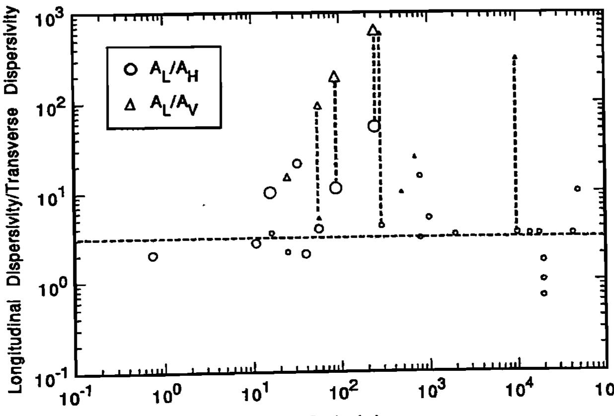
A critical review of dispersivity observations from 59 different field sites was developed by compiling extensive tabulations of information on aquifer type, hydraulic properties, flow configuration, type of monitoring network, tracer,...
moreA critical review of dispersivity observations from 59 different field sites was developed by compiling extensive tabulations of information on aquifer type, hydraulic properties, flow configuration, type of monitoring network, tracer, method of data interpretation, overall scale of observation and longitudinal, horizontal transverse and vertical transverse dispersivities from original sources. This information was then used to classify the dispersivity data into three reliability classes. Overall, the data indicate a trend of systematic increase of the longitudinal dispersivity with observation scale but the trend is much less clear when the reliability of the data is considered. The longitudinal dispersivities ranged from 10 -2 to 10 4 m for scales ranging from 10 -1 to 105 m, but the largest scale for high reliability data was only 250 m. When the data are classified according to porous versus fractured media there does not appear to be any significant difference between these aquifer types. At a given scale, the longitudinal dispersivity values are found to range over 2-3 orders of magnitude and the higher reliability data tend to fall in the lower portion of this range. It is not appropriate to represent the longitudinal dispersivity data by a single universal line. The variations in dispersivity reflect the influence of differing degrees of aquifer heterogeneity at different sites. The data on transverse dispersivities are more limited but clearly indicate that vertical transverse dispersivities are typically an order of magnitude smaller than horizontal transverse dispersivities. Reanalyses of data from several of the field sites show that improved interpretations most often lead to smaller dispersivities. Overall, it is concluded that longitudinal dispersivities in the lower part of the indicated range are more likely to be realistic for field applications. --+vi•=• Dij at Oxi Oxi i,j= 1, 2, 3 (1) where c is the solute concentration, v i is the seepage velocity component in the xi direction, and Dij are the components of the dispersion coefficient tensor. The fighthand side of (1) represents the net dispersive transport which is presumed to be Fickian, i.e., the dispersive mass flux is proportional to the concentration gradient. Some investigators [e.g., Robertson and Barraclough, 1973; Bredehoeft and Pinder, 1973] alternatively define the dispersion coefficient tensor including the porosity n as D•j =nD ij. When it was clear that D•j was used in a study, we converted to the more common form used in (1). The mean flow direction is taken to be Xl, with vl = v, v2 = v3 = 0. Assuming that xl, x2, and x 3 are principal directions, the dispersivity is simply the ratio of the appropriate component of the dispersive coefficient tensor divided by the magnitude of the seepage velocity, v. To distinguish the field-scale dispersivities from laboratory values, the field-scale values are designated by the uppercase letter A [see Ge!har and Axness, !983] and, to allow for anisotropy of transverse dispersion, a third dispersivity coefficient is used as follows: Dll = ALV D22 = Arv D33 = Avv (2) where A t• is the longitudinal macrodispersivity (field scale), and A T is the horizontal transverse macrodispersivity, and A v is the vertical transverse macrodispersivity. The classical equation (1) with macrodispersivities (2) is standardly used for applied modeling of field-scale solute transport. The macrodispersivities are considered to be a property of some region of the aquifer. Although the macrodispersivity may be a function of space, in most applications it is assumed constant over a region of the aquifer that encompasses the entire plume both horizontally and vertically. Real solute plumes are observed to be threedimensional [LeBlanc, 1982; Perlmutter and Lieber, 1970; MacFarlane et al., 1983] and often of limited vertical extent. Although the classical equation is three-dimensional, the two-dimensional form is most commonly applied. Reasons for the use of the two-dimensional form of the equation include lack of three-dimensional data and in the case of Geophys. Res., 72(16), 4081-4091, 1967. Wilson, L. G., Investigations on the subsurface disposal of waste effluents at inland sites, Res. Develop. Progress Rep. 650, U.S.


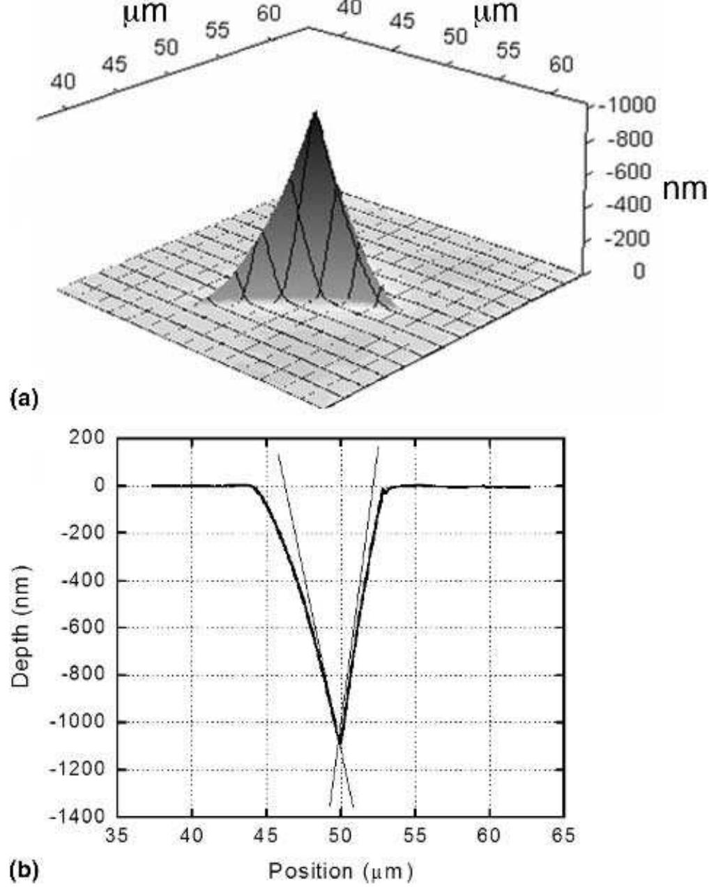
![FIG. 3. Concepts used to understand and define the effective indenter shape (from Ref. 35). The ideas underlying the effective indenter shape are outlined in Fig. 3. The basic principles are derived from observations gleaned from finite element simulations of indentation of elastic—plastic materials by a rigid conical indenter with a half included angle of 70.3°.*° During the initial loading of the indenter [Fig. 3(a)], both elastic and plastic deformation processes occur, and the indenter conforms perfectly to the shape of the hardness impres-](https://figures.academia-assets.com/36597907/figure_003.jpg)


![left end of the beam. The crack iS assumed to open at the section to the right, which is the section of symmetry. Mgis the moment which gives 03] = ft, where o3] is the stress at point 31. Mp would be the failure moment if the material were elas- tic and perfectly brittle. When M is raised above Mj the crack starts Opening at point 31. At that point we introduce a force corresponding to the relation between stress ao and crack width w according to Fig. 4c. With this new finite element system we can calculate the stress at point 32 and we can determine that value M = Mj), which gives a stress 032 = f,. We can now introduce another force at point 32 and calculate a moment M = M2» giving 033 = ft etc. By proceeding in the same way we get a relation between crack depth and applied moment according to Fig. 7.](https://figures.academia-assets.com/32236147/figure_004.jpg)


![Gesign area tnat ?s available for the construction of the fillet. For the sake of comparison, a design optimization was also carried out for the case of rigidity that is linear in the design variable, as for variable thickness sheets, cf. Section 2. Suc design problems have been studied in detail in [51], and are very well-behaved problem: Figure 10 shows results for this type of problems and illustrates that this representation stiffness gives a good indication of the two-dimensional optimal shape for high volum fractions, while for low volume fractions it is difficult to interpret the results so as to define two-dimensional shape. This is, of course, not surprising as we are dealing with a tru three-dimensional problem that just happens to have a two-dimensional model. That is th variable thickness is a hidden three-dimensional feature. However, the design of variab] thickness sheets does indeed give well-defined shapes as three-dimensional structures. The testing of the design method using composite materials has been carried out for variou different formulations that all relate to the description of the method given in Section 4. Tw](https://figures.academia-assets.com/33987352/figure_008.jpg)


![“MVE PUL HO ‘216 O18 SOUIN[OA ‘sUdIsap podumn] SuNNses oy) UUINTOS pueYy-7Yy3IE ‘SuIduIN] 0} JO y[NsAa1 SMOYs UUIN[OS pueY-2T] °psjej03 aq WED Jey) Sajoy arenbs se sploA YIM Y aseD “ssodoid Suiduiny ayy Jo syNsey “pT “By](https://figures.academia-assets.com/33987352/figure_013.jpg)

![WHT EM VVELU GE SELULOsS LM MIC Gi LU Ue CHU Le PCeLivy of the evaluation. Note, however, that the coefficient of deter- mination is limited in that it standardizes for differences be- tween the observed and predicted means and variances since it only evaluates linear relationships between the variables. It can be easily demonstrated that if P, = (AO, + B) for any nonzero value of A and any value of B, then R? = 1.0. Thus R? is insensitive to additive and proportional differences be- tween the model simulations and observations [see Willmott, 1984]. Large values of R? can be obtained even when the model-simulated values differ considerably in magnitude (i.e., values of B that differ significantly from 0.0) and variability (i.e., values of A that differ significantly from 1.0). Clearly, in such cases, a model would exhibit serious flaws that should preclude the attribution of a “perfect” designation. These lim- itations in the coefficient of determination and other correla- tion-based measures are well documented [cf. Willmott, 1981; Moore, 1991; Kessler and Neas, 1994; Legates and Davis, 1997], although such measures still have been used recently to pro- vide, for example, an assessment of climate change detection [e.g., Santer et al., 1995; Hegerl et al., 1996; Santer et al., 1996] and hydrological and hydroclimatological applications (see McCuen and Snyder [1975] and Willmott [1984] for some ex- amples).](https://figures.academia-assets.com/43785224/figure_001.jpg)
![where j represents an arbitrary power (i.e., a positive integer). Note that the original index of agreement d developed by Willmott [1981] becomes d, using this notation.](https://figures.academia-assets.com/43785224/figure_002.jpg)
![where O’ is the baseline value of the time series against which the model is to be compared. It usually is a function of time and, in some applications, may be a function of other variables as well. Consequently, d{, is useful in that its interpretation is more conventional, as it more closely follows the interpretation Garrick et al. [1978, p. 376] further argued that the assump- tion of comparing the model to the observed mean was “un- necessarily primitive.” Better methods exist to define the base- line against which a model should be compared. For example, persistence or averages that vary by season or another time period (i.e., a climatology) may provide a more appropriate baseline for most hydrological or hydroclimatological studies than simply the average of the entire time series. Thus both E, and d, can be rewritten in a “baseline adjusted” form as](https://figures.academia-assets.com/43785224/figure_003.jpg)

![Figure 1. Time series of monthly potential evapotranspiration estimated by the Thornthwaite [1948], Jensen and Haise [1963], and van Bavel [1966] methods compared with observations (measured pan evaporation multiplied by a pan coefficient of 0.76). Data were taken from January 1981 through December 1983 for southern Louisiana (data from McCabe and Muller [1987]).](https://figures.academia-assets.com/43785224/figure_005.jpg)

![Figure 3. Observed and modeled monthly runoff (precipitation runoff modeling system) for the East River Basin in southwestern Colorado from October 1972 through September 1989 (data from McCabe and Hay [1995]).](https://figures.academia-assets.com/43785224/figure_007.jpg)


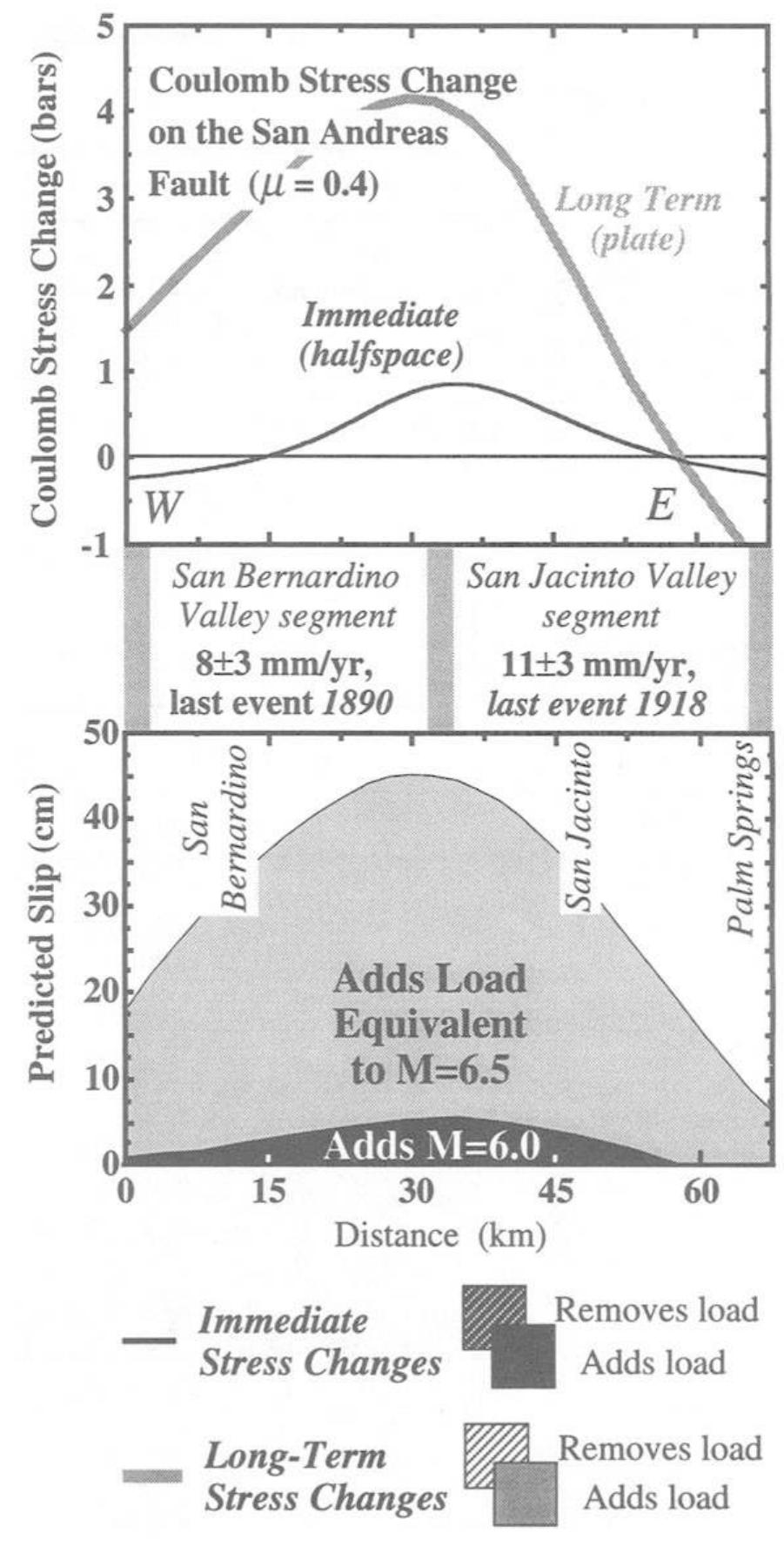
![Figure 13. The largest Coulomb stress changes at depths between 0 and 12.5 km caused by the Landers, Big Bear, and Joshua Tree earthquakes, shown with the first 25 days of seismicity from Hauksson ef al. (1993). Also shown are the largest two aftershocks to occur during the following 8 months, the 17 November 1992 M, = 5.3 and 4 December 1992 M, = 5.1 shocks. Few aftershocks are seen near Indio in the Coachella Valley where the San Andreas was loaded by the Lan- ders earthquake and, to a lesser extent, by the Imperial Valley (Hanks and Allen, 1989), Elmore Ranch, and Su- perstition Hills (Hudnut et al., 1989) events [the effect of these earthquakes is shown in Stein et al. (1992)]. The lack of earthquakes near Indio appears to be an ex- ception to the observation that Coulomb stress rises are accompanied by at least some activity, although trig- gered surface slip was seen at several points between Indio and the southeastern end of the San Andreas (D. Ponti, personal comm., 1992). Landers aftershocks could be absent in the Coachella Valley because the total stress there is lower, because the fault is locally tougher, or because modulus contrasts modify the Coulomb stresses. We examined the effect of a low-modulus Mojave tec-](https://figures.academia-assets.com/50188658/figure_013.jpg)


![diffusion, then (29) takes on a relatively simple form which can be evaluated exactly; this involves extensive manipula- tions which are available from Gelhar and Axness [1981]. The results, are seen to agree, to lowest order in ¢, with the asymptotic results (33) and (36), when a, = az. Figure 1 shows a comparison of the exact and aproximate results; this indi- cates that the approximate solution is adequate for « < 0.01. Note that the ratio of transverse to longitudinal macroscopic dispersion is ¢/3, which will be very small under typical conditions.](https://figures.academia-assets.com/48725868/figure_004.jpg)


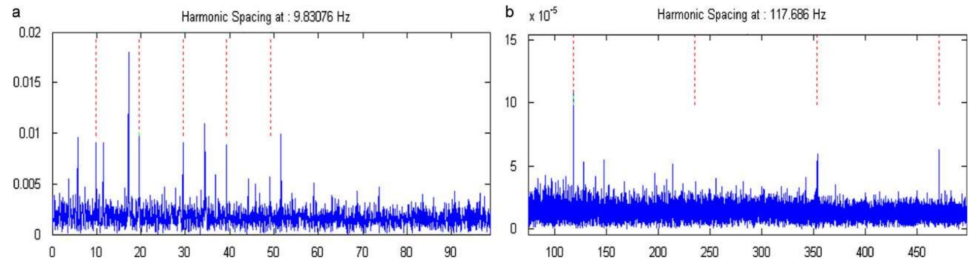
![Fig. 3. Typical modulating signal from the effect of an extended inner race fault on a gear signal. However, the way of modelling the random variation in pulse spacing in Ref. [13] (model 1) was later found to be incorrect, and in [14] a more correct model (model 2) was proposed. As illustrated in Fig. 4, the variation in model 1 was Model 1 For localised faults, the question arises as to the correct way to model the random spacing of the impacts. Perhaps the first publication to model bearing fault signals as cyclostationary was [12], but the results were not very convincing, possibly because the main resonances excited by the faults may have been outside the measured range up to about 6 kHz. Results are shown below (Fig. 18) where localised faults on a very similar sized bearing only manifested themselves at frequencies above 8 kHz. Good results were obtained in [13], by modelling the vibration signals from localised bearing faults as CS2 cyclostationary. Random variable is the jitter Of. around each period](https://figures.academia-assets.com/42711119/figure_003.jpg)

![Fig. 7. Spectral correlation for a mixture of first and second-order cyclostationarity, illustrated using modulation by gear and bearing signals: (a) gearmesh modulation by a gear signal; (b) gearmesh modulation by an extended inner race bearing fault; and (c) spectral correlation for case (b). From [14]. Fig. 6. Spectral correlation and spectrum of the squared envelope for a local inner race bearing fault. BPFI=120 Hz, shaft speed=9.5 Hz.](https://figures.academia-assets.com/42711119/figure_005.jpg)


![Fig. 10. Schematic diagram of self-adaptive noise cancellation used for removing periodic interference (gear) leaving random signal (bearing). In Ref. [22] SANC was likened to prediction theory, and it was pointed out that the asymptotic result in Fig. 11 is in agreement with the analytical result that the bandwidth of the SANC filter is the reciprocal of the period of the frequency being separated, and the filter characteristic is almost identical to that for the equivalent comb filter for synchronous For fewer than 12 spectral components some saving can be made, but above this the minimum order corresponds to approximately one period of the frequency spacing. Ho recommends that the order should be at least double the minimum for best results.](https://figures.academia-assets.com/42711119/figure_009.jpg)
![Fig. 11. Minimum filter order vs number of discrete spectrum components. averaging (e.g. Fig. 13). In [23] it was also pointed out that it can be advantageous to vary the convergence factor exponentially, to start with a larger value and reduce it as the convergence proceeds.](https://figures.academia-assets.com/42711119/figure_010.jpg)
![Fig. 12. Example of enhancement of an outer-race fault signal in a gearbox: (a) measured vibration signal, (b) extracted periodic part (gears), an (c) extracted non-deterministic part (bearing). The filter characteristic corresponding to this expression is shown in Fig. 13 ([25]) for the case where N=8, and is seen to be a comb filter selecting the harmonics of the periodic frequency. The greater the value of N the more selective the filter and greater the rejection of non-harmonic components. The noise bandwidth of the filter is 1/N, meaning that the improvement in signal/noise ratio is 10 log;, N dB for additive random noise. For masking by discrete frequency signals, it should be noted that the characteristic has zeros which move with the number of averages, so it is often possible to choose a number of averages which completely eliminates a particular masking frequency. The above characteristic is for an infinitely long time signal x(t), and in Ref. [25] it is shown that for the practical situation of a finite length of signal with](https://figures.academia-assets.com/42711119/figure_011.jpg)
![Fig. 13. Filter characteristic corresponding to 8 synchronous averages (from [25]).](https://figures.academia-assets.com/42711119/figure_012.jpg)


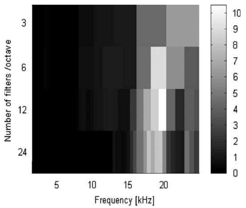
![Fig. 19. (a) PSD spectra with the different window lengths and (b) SK calculated for the indicated window length in samples (from [35]](https://figures.academia-assets.com/42711119/figure_017.jpg)
![Fig. 20. Kurtogram for a weak bearing fault in a gearbox [35]. Nw is window length defining spectral resolution. SK is spectral kurtosis. Maxima are projected onto each plane.](https://figures.academia-assets.com/42711119/figure_018.jpg)
![Fig. 21. (a) Optimal bandpass filter compared with SK at N,=44 and (b) outer race fault signal obtained using the filter of (a) (from [35])](https://figures.academia-assets.com/42711119/figure_019.jpg)
![Fig. 22. Combinations of centre frequency and bandwidth for the 1/3-binary tree kurtogram estimator [37].](https://figures.academia-assets.com/42711119/figure_020.jpg)
![‘ig. 23. Comparison of the fast kurtogram with the full kurtogram for an impulsive signal from loose parts monitoring [37] time averages in Eq. (21). This is rather similar in principle to the FFT algorithm and even more similar to the “discret wavelet packet transform” (DWPT). In Ref. [37], an even finer decomposition is proposed, based on a “1/3-binary tree’ where each halved-band is further split into 3 other bands, thus producing a frequency resolution as illustrated in Fig. 22 in the sequence 1/2, 1/3, 1/4, 1/6, 1/8, 1/12,...,2~*~', with corresponding “scale levels” k=0, 1, 1.6, 2, 2.6,..., that enforce | similarity in notation with the DWPT transform. It should be noted that, however, in addition to providing a fine resolution than allowed by the DWPT (actually limited to integer values of k only), the proposed solution also has mucl better filtering characteristics as demonstrated in Ref. [37].](https://figures.academia-assets.com/42711119/figure_021.jpg)
![Fig. 24. Example of advanced wavelet denoising: (a) raw vibration signal; denoised signal using NeighCoeff shrink based on (b) DTCWT; (c) DW (discrete wavelet transform), and (d) SGWT (second-generation wavelet transform). From [43].](https://figures.academia-assets.com/42711119/figure_022.jpg)
![Fig. 25. Procedure for envelope analysis using the “Hilbert transform” method [45].](https://figures.academia-assets.com/42711119/figure_023.jpg)


![Fig. A1. Example of amplitude modulated white noise (from Antoni [10]): (a) time signal over four periods of cyclic frequency; (b)two-dimension. autocorrelation function vs time (sample) n and time lag t. is a periodic function of time, ie. Ryx(t,t)=Rxy(t+T,t) (this is not to be confused with the stationary enforce autocorrelation function computed as the time averaged <Rx(t,T)> =Rxx(t)). A simple example is provided by a whit noise modulated by a periodic amplitude, as illustrated in Fig. A1(a). Note that, in spite of the periodic modulation, this i still a completely random signal. The autocorrelation function, by virtue of the second-order non-linearity it introduce:](https://figures.academia-assets.com/42711119/figure_035.jpg)
![Fig. A2. Spectral correlation for the case of Fig. Al(a) (from [10]). where X;(f) stands for the Fourier transform of signal x(t) over an interval of duration T. Formula (A3) is probably most convenient when it comes to estimate the spectral correlation from finite-length measurements since it is easily amenable](https://figures.academia-assets.com/42711119/figure_036.jpg)
![Fig. A3. Wigner-Ville spectrum for the case of Fig. A1(a) (from [10]).](https://figures.academia-assets.com/42711119/figure_037.jpg)

![Fig. B3. Use of tracking to avoid smearing of shaft speed related components. Fig. B2. Comparison of frequency characteristics for interpolation at different orders (from [49]).](https://figures.academia-assets.com/42711119/figure_039.jpg)


![1. The tracer test was either ambient flow with known input, diverging radial flow, or a two-well pulse test (without recirculation). These three test configurations produce break- through curves which are sensitive to the dispersion coefficient and appear to work well in field applications [Welty and Gelhar, 1989]. The radial converging flow test is generally considered less satisfactory than the diverging test because breakthrough curves at the pumping well for the converging test frequently exhibit tailing, which complicates the interpre- tation of these tests. Some researchers attribute this behavior to two or more discrete geologic layers and try to reproduce the observed breakthrough curve by superposition of break- through curves in each layer, where the properties of each layer may differ [e.g., Ivanovitch and Smith, 1978, Sauty, 1977]. The problem with this interpretation is that there are typically numerous heterogeneities on a small scale that cannot be attributed solely to identifiable layers. One possible expla- nation of the tailing in radial convergent tests is sometimes termed ‘‘borehole flushing,’’ where the tail of the breakthrough curve is attributed to the slow flushing of the input slug of tracer out of the injection borehole by the ambient groundwater flaw. Goblet [1982] measured the slow flushing of tracer out of the values that do not fall into the high or low groups. These classifications do not place strict numerical confidence limits on reported dispersivities, but rather are intended to provide an order-of-magnitude estimate of the confidence we place on a given value. In general, we consider high-reliability dispersivity values to be accurate within a factor of 2. Low-reliability values are considered to be no more accurate than within 1 or 2 orders of magnitude. Intermediate reliabil- ity falls somewhere between the extremes. We wish to make a distinction between the judgment of the reliability of the reported dispersivity and the worth of a study. Often, the Purpose of a study was for something other than the deter- mination of dispersivity. Our classification of dispersivity is not intended as a judgment on the quality of a study as 2 whole, but rather to provide us with some criteria with which to screen the large number of data values obtained. By then examining the more reliable data, conclusions which evolve from the data will be more soundly based and alternative interpretations may’ become apparent.](https://figures.academia-assets.com/48725864/table_008.jpg)


![Fig. 1. A) CaO-Al,03-SiO, ternary diagram of cementitious materials, B) hydrate phases in the CaO-Al,03-SiO2 system. Note that in the absence of carbonate or sulfate, C;AHg will be more stable than the AFm phases. Most of the available studies on the properties of blended systems composition and the hydrates formed as well as their impact on t processes taking place in the hydration of Portland cements (PC) well known (see e.g. the comprehensive book of Taylor [1]). clinker phases hydrate at various rates resulting mainly in t formation of C-S-H, portlandite, ettringite and AFm phases. T system where the hydration of the Portland cement and hydrauli reaction of the SCM occur simultaneously and may also influence t! reactivity of each other. The reaction of most SCMs is slower than t ong-term development of such systems is insufficient. The main are The blending of SCMs with Portland cement leads to a more complicated focus on mechanical or durability aspects of a specific fly ash or slag. Our knowledge about fundamental connections between the overall ne ne ne 1c ne ne reaction of the clinker phases and difficult to follow as many SCMs](https://figures.academia-assets.com/63535708/figure_001.jpg)

![Fig. 3. SEM-BSE from a 60% Portland cement-40% slag blend (B-S1) hydrated for 1 year From Kocaba [13]. The hydrate assemblage observed experimentally in Si02—-PC blends agrees well with the modelling results shown in Fig. 5. It consists of mainly C-S-H, ettringite, AFm phases [20-22] and a reduced quantity of portlandite [22-25]. The blending of PC with >24wt% silica fume resulted after longer hydration times in the entire consumption of portlandite with ettringite and C-S-H with a reduced Ca/Si ratio as the only hydrate phase observed ([22,23,25,26], Fig. 6). As the silica fume continued to react, the low pH values and the absence of portlandite destabilized the monocarbonate with time [26,27]. The calculations in Fig. 5 indicate, that upon further replacement of PC by silica fume (or upon further reaction of the silica fume), ettringite will become unstable. The dissolution of](https://figures.academia-assets.com/63535708/figure_003.jpg)
![‘ig. 4. Ca/(Si+ Al) ratio in Portland cement (B) and 60% Portland cement-40% slag blends (B-S1; B-S8) hydrated up to 1 year. The lines indicate the Ca/(Si+ Al) ratio of the pure slag slags 1 and 8). (ram Kocaha [13].](https://figures.academia-assets.com/63535708/figure_004.jpg)
![Fig. 5. Modelled changes in hydrated Portland cement upon blending with SiOz, assuming complete reaction of the Portland cement (CaO 60, SiO, 22, Al,03 4.6, Fe203 2.7, MgO 1.9, Na20 0.3, K20 1.0, SO3 3.2, CO2 2 wt.%) and SiO. Fig. 5 illustrates an important aspect related to the partial replacement of Portland cement with SCMs — the decrease in the total volume of hydrates formed. This should mean that blended pastes have higher total porosities than pure PC pastes. This seems paradox as it is well established that PC-SCM blends can develop higher strengths and lower permeabilities than plain PC pastes (e.g. 29]). This poses the question as to whether the effective density, or space filling capacity of C-S-H in blended pastes is the same as in plain Portland pastes. Measurements indicate that blended systems show often equal or even higher total porosities than pure PC pastes, but a refined pore structure [30-33]. In particular, slag-PC pastes have been observed to contain more fine pores and less coarse capillary pores than PC pastes, resulting in a reduced permeability 30,32]. Fly ashes consist mainly of SiOz, but can contain also significant quantities of Al,O3. The amount of CaO is limited but highly variable depending on the origin of the fly ash (e.g. [1], Fig. 1). The ASTM C618 standard differentiates high calcium Class C-fly ashes and low-calcium Class F ashes. As the latter are the most abundant, the following discussion focuses on Class F fly ash. The blending of Portland cement with fly ash results in the reduction of the total amount of portlandite in the hydrated mixture, somewhat less pronounced than for silica fume as (i) the reactivity of fly ash is very limited and (ii) as the CaO in the fly ash is an additional source of calcium. Class F fly ashes contain between 15 and 35% alumina, so the blending of PC with such fly ash results in high amounts of Al-rich phases. As systematic information about the Al-uptake by C-S-H are still missing (see also discussion in Appendix A), the high aluminium content in the system, coupled with a potentially high aluminium uptake in C-S-H introduces a consider- able error in the thermodynamic calculations. For our calculations, a constant Al/Si of 0.1 in C-S-H was assumed. The results indicate, in the presence of moderate amounts of fly ash, the destabilization of](https://figures.academia-assets.com/63535708/figure_005.jpg)
![Fig. 6. Phase composition observed by XRD in a hydrated Portland cement, a CEM III/B blended with 10% SiOz and a CEM I blended with 40 wt.% SiO after one year of hydration. Graph modified from [26].](https://figures.academia-assets.com/63535708/figure_006.jpg)


![Fig. 9. Hydration of 100% PC compared to 70% PC with 30% fine quartz filler. The rate of heat evolution is normalised to the PC content [53]. The quartz, as it does not react significantly, gives more space for hydration product of the PC so the acceleration period is prolonged. Recent results from Fernandez [53] and Kocaba [13] illustrate these effects. Figs. 9 and 10 show the heat evolution curves for blends with quartz filler and silica fume compared to reference cements. In both cases the heat evolution is normalized to the amount of clinker phases present. Quartz was chosen as a nominally inert material, although there may be some reaction of an amorphized surface layer](https://figures.academia-assets.com/63535708/figure_009.jpg)
![Fig. 10. a) 100% PC compared to 90% PC with 10% silica fume, the fine particles of silica fume act as nucleation sites to give a steeper acceleration and higher maximum rate of heat evolution [56]. Panel b shows simulation results in which the number of nucleation sites increased by 30% [57].](https://figures.academia-assets.com/63535708/figure_010.jpg)
![Fig. 11. Heat evolution for PC blended with corundum, rutile or quartz. Fineness corundum 5.4 m? g~!; rutile 9.1 m? g~!; quartz 0.76 m? g~!. Adapted from [58]. The technique which has been used most widely to try and measure the reactions of SCMs in blended systems is selective dissolution [62]. The intention of such methods is that the unreacted clinker phases and the hydrates from the clinker and slag reaction are dissolved, leaving only the unreacted slag or fly ash as a residue. Study of residues by X-ray diffraction and SEM reveals that significant amounts of clinker and hydrate phases remain after dissolution [13,62-64]. It is claimed that the effects of incomplete dissolution can be corrected for. However, recent independent work by two of the authors of this paper [13,63-65] indicates that large, non-quantifiable systematic errors remain as different assumptions lead to large differences in the quantity of FA or slag reacted. This probably explains why different authors report very different amounts of slag](https://figures.academia-assets.com/63535708/figure_011.jpg)


![Fig. A1. Aqueous concentrations and mole fractions of the C-S-H solid solution end-members (jennite-tobermorite) as a function of the Ca/Si ratio. The presence of portlandite and amorphous SiOz is indicated by horizontal lines (out of scale). Modified from [84,106].](https://figures.academia-assets.com/63535708/figure_014.jpg)


