scholarships were essential for the realization of this project. To Prof. Dr. Fernando Martini Catalano, for the friendship, support, knowledge and experience shared with me throughout all these years, either as teacher when I was an...
morescholarships were essential for the realization of this project. To Prof. Dr. Fernando Martini Catalano, for the friendship, support, knowledge and experience shared with me throughout all these years, either as teacher when I was an undergraduate student, either as a supervisor during the execution of the research, or as my supervisor during my teaching internship. To Prof. Dr. José Antônio Garcia Croce, who kindly gave his massive contribution in the implementation and maintenance of the high voltage high frequency AC power supply, without which the experiments of this research could not have been carried out. To the technicians José Claudio Pinto de Azevedo, Mário Sbampato and Osnan Ignacio Faria, for their friendship, solicitude, aid and shared knowledge in the manufacture, assembly, maintenance and operation of the necessary equipment for the experiments. To Gisele Aparecida Poppi Lavadeci, secretary of the Department of Aeronautical Engineering, who was always available to assist me with the bureaucracies, printings or just to talk and take a coffee. To the São Carlos School of Engineering Library staff, for checking the typesetting and the referencing style. To my friends and laboratory colleagues, the engineers


![Fig. 7. LHS designs with significant differences in terms of uniformity [36]. While LHS represents an improvement over unrest- ricted stratified sampling [37] it can provide sampling plans with very different performance in terms of uniformity (issue b) measured by, for example, max- imum minimum-distance among design points, or by correlation among the sample data. Fig. 7 illustrates this](https://figures.academia-assets.com/48438222/figure_007.jpg)


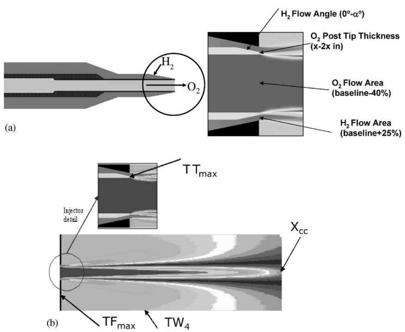


![Fig. 13. Main factor (S;,) influence on objective variability: (a) TFinax, (b) TWa, (c) TTinax and (d) Xec. While it is well established that variations in injector geometry can have a significant impact on performance and environmental objectives such as combustion chamber wall and injector face temperatures and heat fluxes [107], these sensitivities are seldom quantified. As shown in Vaidyanathan et al. [10], once surrogates become available, these sensitivities can be computed using Sobol’s method (Section 6). The sensitivity information cited above can be used for screening purposes and therefore, ease the search for optimum designs. In fact, surrogate models that included only essential variables (with the non essential](https://figures.academia-assets.com/48438222/figure_014.jpg)


![Different techniques in sensitivity analysis, and application examples, can be found in the works of Iman and Helton [68], Kleijnen [69] and Frey and Patil [70], and references therein “Independent from assumptions about the model being linear, etc. >There are exceptions e.g., the Spearman rank-order correlation coefficient.](https://figures.academia-assets.com/48438222/table_003.jpg)


![In order to avoid interpenetration of the crack faces, the following condition is introduced: Using 5™** in the constitutive equation, the irreversibility of damage is taken into account. This is shown in Figure 2: if the relative displacement decreases, the point unloads elastically towards the origin with a reduced, secant, stiffness (point 3 in Figure 2). The irreversible, bi-linear, softening constitutive behaviour for single-mode loading shown in Figure 2 can be defined as [23,39,44]:](https://figures.academia-assets.com/49707537/figure_003.jpg)


![Table 1. Properties for AS4/PEEK [55,58]. The experimental tests were performed by Reeder and Crews [55] at different Gy/G ‘atios (0.0, 0.2, 0.5, 0.8 and 1.0), ranging from pure Mode I loading to pure Mode | oading*. The specimens are 102 mm-long, 25.4mm-wide, with two 1.56mm-thick arm [he material properties are shown in Table 1, and a penalty stiffness K= 10° N/mm? ised. The initial delamination length of the specimens (ao) and the mixed-mode fractur oughness obtained experimentally [55] are shown in Table 2. It is worth noticing that th nitial delamination length for the ENF test specimen, ag =39.3mm, leads to stab ropagation of the delamination. For the material and geometry used here, it was show xy Reeder and Crews [55] that for initial delamination lengths smaller than 35m instable propagation occurs, because G exceeds Gc as the delamination grows. Models using 150 decohesion elements along the length of the specimens, and](https://figures.academia-assets.com/49707537/figure_007.jpg)


![?The load—displacement relations experimentally determined for the different mode ratios are not reported in [55]. This information was provided by the author of the experiments [58].](https://figures.academia-assets.com/49707537/table_001.jpg)
![Table 3. Experimental [55,58] and numerical maximum loads.](https://figures.academia-assets.com/49707537/table_002.jpg)

![Table 6. Mode I and Mode II load components. APPENDIX B: DETERMINATION OF THE LOAD-POINT DISPLACEMENT The information available from the MMB test relates the load to the displacement of the load-point (Figure 5). Since the lever is not simulated in the numerical models, it is necessary to calculate the load-point displacement using the information available from the numerical models of the MMB test specimens. The load-point displacement, Arp, is obtained from the pure mode displacement components, A; and Ay, as [60]:](https://figures.academia-assets.com/49707537/table_005.jpg)


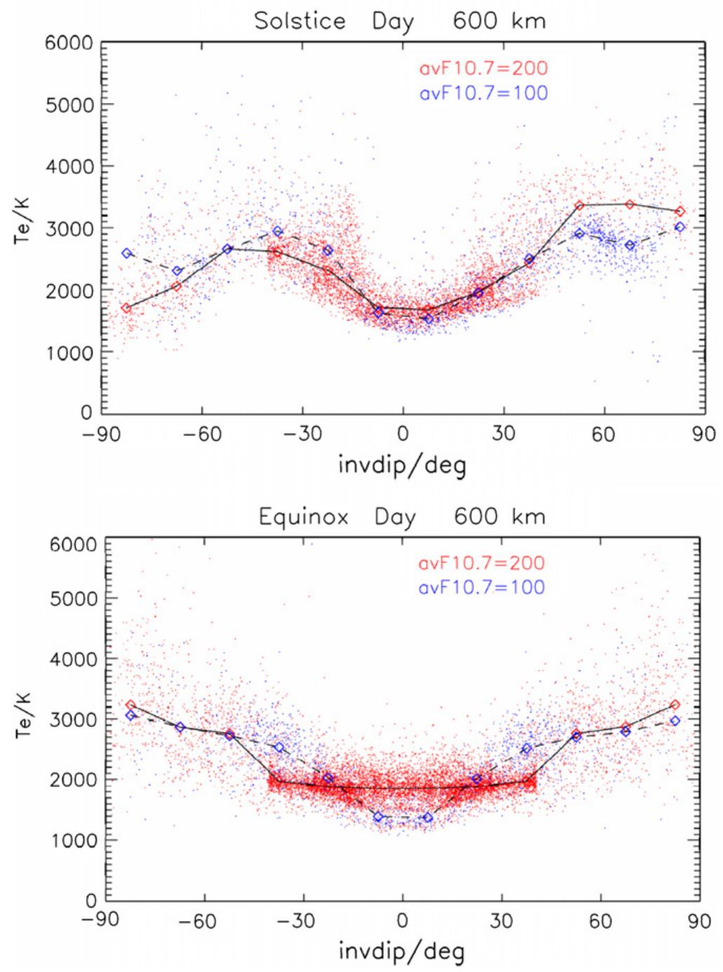


![IRI, IRI-2001; cor, IRI-2007a; NeQ, IRI-2007b; TTS, Triskova et al. (2006) model. Mean and standard deviation (std) of the data-model differences [(data-model)/data] for the different Alouette and ISIS data sets (n = number of profiles) Table 1](https://figures.academia-assets.com/73092299/table_001.jpg)


![where P; and D, are the production and destruction terms from the turbulent kinetic energy equation in the original SST turbu- lence model and Yer is the effective intermittency obtained from Eqs. (24)-(26). 3.4 Coupling With the Turbulence Model. The new transi- tion model has been calibrated for use with the SST turbulence model Menter [12]. The transition model is coupled with the tur- bulence model as follows:](https://figures.academia-assets.com/46899821/figure_009.jpg)

![Fig. 8 Skin friction (Cf) for the T3B test case (FSTI=6.5%) Test cases presented in this paper include the ERCOFTAC [1,2] T3 series of flat plate experiments and the well-known Schubauer and Klebanof [18] flat plate experiment, all of which are com- monly used as benchmarks for transition models. The first three cases (T3A-, T3A, and T3B) have zero pressure gradient with free-stream turbulence levels of 1%, 3% and 6% that correspond to transition in the bypass regime. The Schubauer and Klebanof [18] test case has a low free-stream turbulence intensity and cor- responds to natural transition. The T3C4 test case consists of a flat plate with a favorable and adverse pressure gradient imposed by](https://figures.academia-assets.com/46899821/figure_011.jpg)
![Fig. 10 Skin friction (Cf) for the Schubauer and Klebanof [18] test case (FSTI=0.18%)](https://figures.academia-assets.com/46899821/figure_012.jpg)


![Fig. 13 Normalized wall friction velocity distributions (u,/U, on the suction side of the Genoa cascade Ubaldi [19] The authors would like to acknowledge the support and techni- cal contributions from Dr. William Solomon at GE Aircraft En- gines. The model development and validation at ANSYS CFX](https://figures.academia-assets.com/46899821/figure_016.jpg)
![Table 1 Summary of all test case inlet conditions low turbulence intensities, the new correlation has been designed to predict a large increase in Reg, whenever a favorable pressure gradient is present. This is based on Drela’s [14] e" model, which indicates that small favorable pressure gradients will cause a large increase in Re». Based on the Fashifar and Johnson [15] data, the effect appears to be reduced as the freestream turbulence intensity increases and the new correlation is designed to reflect this. The new empirical correlation is defined as follows:](https://figures.academia-assets.com/46899821/table_001.jpg)


![Fig. 3. Distribution of the pressure coefficient CP on the surface of a 2-D circular cylinder of radius r = 6.6, and center- to-center distance H/r = 20. The stagnation point is located at 0 = 180°. The LBE result denoted by symbol x is obtained with t = 0.6 and Re = 40. The solid line is the result obtained by using a 3-D multi-block, body-fitted grid, and pressure- based NS solver with a much finer resolution [96].](https://figures.academia-assets.com/47141313/figure_003.jpg)
![Fig. 5. Schematic for uniform flow over a sphere. where @ accounts for the non-Stokesian effect of the drag. For two types of the boundary conditions at (vy = +H/2,2= +H/2), byym is used to denote the non- Stokesian correction for the case where the symmetry conditions are imposed at (vy = +H/2,z = +H/2) and Punb 18 used to denote the results for the case where the extrapolation for f,’s is used at (vy = +H/2,z = +H/2) in order to simulate the unbounded flow. The D3Q19 model was used. Fig. 4. Drag coefficient for a uniform flow over a column of cylinders over a range of radius r (a) Re = 100 and (b) Re = 10 [96]. For Re = 100, Benchmark solution was given by Fornberg [100].](https://figures.academia-assets.com/47141313/figure_004.jpg)

![Fig. 6. Variation of the non-Stokesian correction factor with sphere radius at Re = 10 [96]. (a) Flow over a single sphere in an unbounded field [96]. (b) Flow over a planer array of spheres. Data are from the LBE simulations.](https://figures.academia-assets.com/47141313/figure_006.jpg)
![Fig. 7. Unsteady flow around a cylinder at Re = 100: instantaneous isobars computed by Filippova and Hanel [83] using local grid refinement technique. The typical interface structure is shown in Fig. 9. The line MN is the fine grid block boundary, while the line AB is the coarse grid block boundary. The coarse block boundary is in the interior of the fine block, and the fine block boundary is in the interior of the coarse block. This arrangement of the interface is convenient for the information exchange between two neighboring blocks. For example, grid Q is an interior lattice node of the coarse block. After the collision step, the values of incoming distribution functions fo(t"*!, Xp), f3(t"*!, Xz) and f4(t’*!, Xz) from boundary nodes D, E, and F, respectively, are needed in order to _ obtain filt™!, XQ), At! XQ) and fa(e"t!, Xq) at the end of A flow over an asymmetrically placed cylinder in the channel [103] was calculated with the grid refinement](https://figures.academia-assets.com/47141313/figure_007.jpg)
![Fig. 8. Unsteady flow around a cylinder at Re = 100 computed by Filippova and Hanel [83]. Coefficients of drag Cp and lift C, and pressure difference Ap between the front and end points of cylinder vs. the number of time steps in coarse grid: solid lines—boundary- fitting conditions; dashed lines—bouncing-back conditions; straight dotted lines—bounds of reference values Cp max; CL max} Ap/(to + T/2) [103]. Reprinted from Journal of Computational Physics, Vol. 147, Filippova and Hanel, Grid refinement for lattice-BGK models, 219-228 (1998), with permission from Elsevier Science.](https://figures.academia-assets.com/47141313/figure_008.jpg)
![Fig. 9. Interface structure between two blocks of different lattice spacing [84].](https://figures.academia-assets.com/47141313/figure_009.jpg)
![Fig. 11. Streamlines in the cavity flow at Re = 100 [84]. Fig. 10. Block layout for a 2-D cavity. Lattice spacing i: reduced by a factor of 8 for graphical clarity [84].](https://figures.academia-assets.com/47141313/figure_010.jpg)
![Fig. 12. Comparison of velocity between results of single- block, multi-block [84] and result of Ghia et al. [105]. (a) Comparison of w-velocity along the vertical line through geometric center and (b) comparison of v-velocity along the horizontal line through geometric center. The computations were carried out using (i) a single- block with uniform lattice (129 x 129) with the walls placed halfway between lattices, and (ii) a multi-block whose layout is shown in Fig. 10. For the multi-block case, in the two upper corner regions, the grid resolution is increased by a factor of 4 comparing with the single- block case. For Re = 100, the streamlines shown in Fig. 11 were obtained from the single-block solution and the pattern is not discernable from those of the](https://figures.academia-assets.com/47141313/figure_011.jpg)
![Fig. 13. Pressure contours in the cavity flow from the single- block LBE simulation [84].](https://figures.academia-assets.com/47141313/figure_012.jpg)
![Fig. 15. Enlarged view of pressure contour in the circled region in Fig. 14 near the intersection of three blocks. The figure demonstrates that the block interface and corner are well handled [84]. To validate the above arguments, pressure and shear stress near the block interfaces were examined. Fig. 15 shows a local, enlarged view of the pressure contour](https://figures.academia-assets.com/47141313/figure_013.jpg)
![Fig. 14. Pressure contours in the cavity from multi-block LBE solution [84] (for the circled region, see Fig. 15).](https://figures.academia-assets.com/47141313/figure_014.jpg)
![Fig. 18. Comparison of Cp between the multi-block simulation and Xfoil [106] calculation as a function of Re for flow over NACAO0012 airfoil. The straight line is the slope according to the laminar boundary layer theory [84]. It is worth pointing out that there is a significant saving in the computational cost using the multi-block method in LBE simulations. There were three different sizes of grids used for the NACA0012 airfoil simulation. There were 1025 x 129=132225 fine grids, 93200 intermediate grids with m = 4, and 139 628 coarse grids (with m= 8 in reference to the finest grids) with a total of about 3.6 x 10° grids in the entire domain. If the fine grid system were used in the entire domain, the number of the grids would be Nyx N= 5698 x 1153~6.57 x 10° which is 18 times more than](https://figures.academia-assets.com/47141313/figure_015.jpg)
![Fig. 16. Shear stress contour. Solid and dash lines represent positive and negative values, respectively [84]. It is also noted that at Re = 500, the value of Cp = 0.1761 compared well with the results reported by](https://figures.academia-assets.com/47141313/figure_016.jpg)
![Fig. 17. Block and lattice layout for flow over NACA 0012. The lattice spacing is reduced by a factor of 32 for graphical clarity [84].](https://figures.academia-assets.com/47141313/figure_017.jpg)
![Fig. 20. Regions of stability and instability in the LBE computation for fully developed 2-D channel flow using the boundary condition of Mei et al. [87], for 4 <i The above three boundary condition treatments all have second-order accuracy for curved boundary. The difference is that the first two need to construct a fictitious fluid point inside the solid wall, and perform a collision step at that node, while the scheme of Bouzidi et al. only requires the known values of f, on the fluid side and no additional collision is required. It is](https://figures.academia-assets.com/47141313/figure_018.jpg)

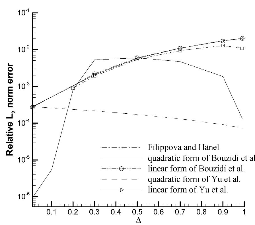
![Fig. 30. (a) Drag coefficient Cp for flow over oscillating zero- thickness flat plate using three different boundary conditions: Filippova and Hanel [83], Bouzidi et al. linear [88], and linear scheme of Yu et al. [89]. (b) Enlarged view of Cp in the circled region in Fig. 30a when A changes from less than 0.5 to larger than 0.5. The figure demonstrates the discontinuity in the temporal variation caused by the Filippova and Hianel [83] and Bouzidi et al.’s boundary treatment [88].](https://figures.academia-assets.com/47141313/figure_030.jpg)

![Fig. 21. Convergence of the factor Q computed by LBE with Bouzidi et al.’s quadratic ( ) and linear interpolation (x ) vs. computational domain size. In the simulation, the fraction of volume occupied by cylinders is kept constant [88]. Courtesy of P. Lallemand.](https://figures.academia-assets.com/47141313/figure_019.jpg)
![Bouzidi et al. [88] presented a simpler boundary condition based on the bounce-back for the wall located at arbitrary position. In their work, both linear scheme and the quadratic schemes were given to obtain fg(x¢, t + dt) which is equivalent to fz(xp,f). The linear version was as follows: Fig. 19. Regions of stability and instability in the LBE computation for fully developed 2-D channel flow using Filippova and Hiinel’s boundary condition [83], for 4 <t [87].](https://figures.academia-assets.com/47141313/figure_020.jpg)
![Fig. 23. Quadratic convergence of the wall-slip velocity using the boundary conditions of Yu et al. [89] in constant pressure- driven channel flow. A Poiseuille flow (see Fig. 22) was used to illustrate the accuracy of the scheme by Yu et al. [89]. This flow is driven by a body force acting as a constant pressure gradient Vp along the x—direction [115]. To assess the computational error of the LBE solution of the velocity, uLpe(y), the following relative L2-norm error is defined:](https://figures.academia-assets.com/47141313/figure_021.jpg)

![Fig. 24. Dependence of relative L-norm error for the boundary conditions of Yu et al. [89] on the lattice resolution H in steady-state pressure-driven channel flow simulations.](https://figures.academia-assets.com/47141313/figure_023.jpg)
![Fig. 25. Variation of (A’ — A) as a function of 1/H for A = 0.01, 0.5, and 0.99 using the linear scheme of Yu et al. [89].](https://figures.academia-assets.com/47141313/figure_024.jpg)
![Fig. 26. Dependence of relative Lj-norm error, defined in Eq. (40), on the lattice resolution H using the linear scheme of Yu et al. [89] in the steady-state pressure-driven channel flow. Fig. 26 shows E% as a function of H for A = 0.01, 0.5, and 0.99. Basically, E has reached the machine error.](https://figures.academia-assets.com/47141313/figure_025.jpg)
![Fig. 27. Slip wall velocity as a function of A using the linear scheme of Yu et al. [89] and Bouzidi et al.’s [88] linear scheme for t=0.502, 0.51, 0.6 and 0.8. The value of (1/v)(dp/dx) is fixed.](https://figures.academia-assets.com/47141313/figure_026.jpg)
![Fig. 28. Slip wall velocity as a function of A using the quadratic scheme of Yu et al. and Bouzidi et al. [88] for t= 0.502, 0.51, 0.6 and 0.8. The value of (1/v)(dp/dx) is fixed. It is further noticed that the largest magnitude of the slip velocity occurs mainly near 4 = 1. This can be attributed to the fact that the interpolation formula given by Eq. (35) has the largest error at A = 1. Thus to reduce the wall-slip velocity, the second-order interpola- tion formula may be used [89]. Fig. 28 shows the wall- slip velocity as a function of A using both quadratic forms of Yu et al.’s scheme and Bouzidi et al.’s scheme for t = 0.502, 0.51 and 0.6. Note that for the quadratic scheme of Yu et al., the slip velocity is amplified by a factor of 100 for t = 0.502 and by a factor of 10 for t = 0.51 in order to show all curves on the same scale. For the low viscosity (t = 0.502) case, the slip velocity using Bouzidi et al.’s quadratic scheme is over 100 times of that using the quadratic formula of Yu et al.](https://figures.academia-assets.com/47141313/figure_027.jpg)
![Fig. 33. Pressure variation (9 —1)/3 at point M at the beginning stage of computation by using the bounce-back inlet condition. Uniform velocity is given as initial condition [116]. Grunau [117] placed the inlet at the lattice node xa (xj = xq and A = 1) as opposed to the lattice halfway link between the grids in which 4 = 0.5 as shown in](https://figures.academia-assets.com/47141313/figure_031.jpg)

![Fig. 34. Schematics of distribution function at inlet for Zou and He’s method [114] at an inlet, wherefo, fs, fs, fs, fo. f7 are known and f\, fo, fg are to be determined. Zou and He [114] proposed a method to specify the inlet boundary condition based on the idea of bounce- back of the non-equilibrium distribution. In this treatment, the inlet is at nodes (xj = xa in Fig. 31a).](https://figures.academia-assets.com/47141313/figure_033.jpg)
![Fig. 35. Pressure variation (p — 1)/3 at point M at the early stage of computation. Uniform velocity is given as initial condition [116].](https://figures.academia-assets.com/47141313/figure_034.jpg)
![Fig. 38. Comparison of the drag coefficient (a) and lift coefficient (b) [116] with the benchmark results given in Schafer and Turek [103].](https://figures.academia-assets.com/47141313/figure_035.jpg)
![Fig. 37. Shear stress profile along y-direction at nodes which are 0.5 lattice unit downstream from the inlet [116]. Fig. 36. Velocity profile along y-direction at nodes which are 0.5 lattice unit downstream from the inlet [116].](https://figures.academia-assets.com/47141313/figure_036.jpg)


![where M is the 9 x 9 matrix transforming F to R. In the vector R, p is the fluid material density, e is the energy, ¢ is related to the square of the energy, j, and j, are the momentum density (or mass flux), g, and q, correspond to the energy flux, and py, and px, correspond to the diagonal and off-diagonal components of the viscous stress tensor. An inherent disadvantage of the SRT d’Humieres [93] presented a 2-D MRT lattice Boltzmann model for the 2-D lattice structure shown in Fig. 1. In this model, a new set of variables R = (p, e, ide Cid Wy Deaenl is introduced and R is related to the set of F = (fo. fis fos fa» fas fs» fo» fr» fay as follows:](https://figures.academia-assets.com/47141313/figure_039.jpg)
![Fig. 42. Comparison of the density profiles at x/L = 0.5125 between the SRT model and MRT model at Re = 1000 [95]. To further develop, a quantitative understanding of the performance of the two models for flow over a flat plate, the streamwise variation of various macroscopic quantities near the plate y/L = 0.0125, which is half-grid](https://figures.academia-assets.com/47141313/figure_040.jpg)
![Fig. 40. Comparison of the relative error in the evolution of the wall shear stress for Stokes first problem between the SRT and MRT models [95]. The flow over a flat plate has a singularity in pressure and stresses at the leading edge of the plate. A schematic of the flow is shown in the insert of Fig. 41. Reynolds number based on the length is Re = UL/v = 1000. Fig. 41 compares the density deviation, p — 1, from the far field value (9 = 1) as a function of y at x/L = 0.0125, which is half grid away from the leading edge, based on the MRT and SRT models under otherwise identical conditions. When there is insufficient numerical resolu- tion for high Reynolds number flows, a non-physical](https://figures.academia-assets.com/47141313/figure_041.jpg)
![Fig. 43. Comparison of the viscous normal stress profiles at x/L = 0.5125 between the SRT model and MRT model at Re = 1000 [95].](https://figures.academia-assets.com/47141313/figure_042.jpg)
![Fig. 41. Comparison of the density profiles near the leading edge (x/L = 0.0125) between the SRT model and MRT model at Re = 1000 [95].](https://figures.academia-assets.com/47141313/figure_043.jpg)
![Fig. 44. Comparison of pressure coefficient as a function of x at y/L = 0.0125 between the SRT model and MRT model [95]. at y/L = 0.0125 as a function of x for solutions based on these two models where p,, is the pressure at the centerline of the inlet. It is noted that the singularity at x =0 resulted in oscillation in C, for about 4-5 grid points after the leading edge in the MRT model.](https://figures.academia-assets.com/47141313/figure_044.jpg)

![Fig. 46. Cavity flow Re = 500 computed by d’Humieres et al. [120], pressure contours at z = 0.5: (a) MRT and (b) LBGK There has been an ongoing effort in construction of stable LBE models and schemes to simulate fully compressible and thermal flows [121-142]. The existing thermal lattice Boltzmann equation (TLBE) models can be classified into three categories. The first category, which is also the simplest approach, is that of passive scalar [121,122,123]. In this approach, the temperature is treated as a passive scalar which is advected by the flow velocity but does not affect the flow fields (density and velocity). The flow fields and the passive-scalar tem- perature are represented by two sets of distribution functions: one simulates the NS equation, and the other simulates the advection-diffusion equation satisfied by](https://figures.academia-assets.com/47141313/figure_046.jpg)

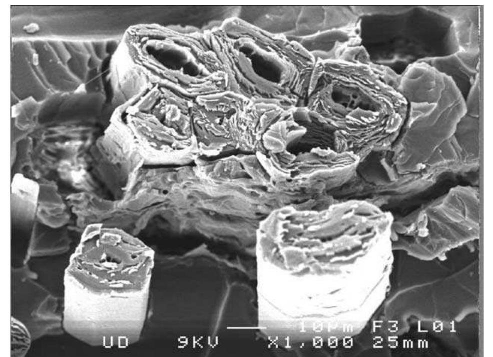
![Fig. 2. Section of a bundle of fibres. The morphological structure of multicellular fibres makes them analogous to the modern reinforced rigid matrix composites. The properties of fibres are also determined by the physical, mechanical and chemica properties of the morphological constituents and_ their interfaces. The polymers involved in the composition of fibres are cellulose, hemicellulose, lignin and pectin. Lignin and pectin act mainly as bonding agents [6]. Typica composition of flax fibres reported by several authors are given in Table | [7—9]. Various parameters can account for the varying accounts of one constituent given by one author to another. These include the species and the variety of the plant, agricultural variables such as soil quality, the weathering conditions, the level of plant maturity, the quality of the retting process [10] and measurement](https://figures.academia-assets.com/43307828/figure_001.jpg)
![Fig. 4. The structure of a flax fibre cell [12-15]. The microstructure of natural fibres is extremely complex due to the hierarchical organisation at different length scale and the different materials present in variable proportions. One has mesoscopic scale, fibre consisting of two cell walls arranged as concentric cylinders with a small channel in the middle called the lumen, which contributes to the water uptake as shown in Figs. 4 and 5 [12-15]. The outer cell wall designed as the primary cell wall is only 0.2 wm thick [16]. The bulk of the fibre is essentially constituted by the layer S2 of the secondary wall cell (Fig. 4). The flax fibre consists of highly crystalline cellulose fibrils spirally wound in a matrix of amorphous hemicellulose and lignin (Fig. 6). They are oriented with a tilt angle of 10° [1,7,16] with the axis of the fibre and hence display a unidirectional structure. A new technique for the](https://figures.academia-assets.com/43307828/figure_002.jpg)

![Fig. 6. Principle of the flax fibre structure. Helical arrangement of fibrils in natural cellulose fibre [3].](https://figures.academia-assets.com/43307828/figure_005.jpg)


![Fig. 17. Young’s modulus plotted as a function of fibre diameter. Finally, it is important to underline that the elastic properties discussed so far relate to low strain rates. For rapid rates, we obtain a dynamic modulus whose order of magnitude is very different [24].](https://figures.academia-assets.com/43307828/figure_016.jpg)


![Examples of composition of flax fibres [7-9] Table 1](https://figures.academia-assets.com/43307828/table_001.jpg)
![Mechanical properties of flax fibre. Values collected from many different publications [4,7,18,21]](https://figures.academia-assets.com/43307828/table_002.jpg)

![Data: elastic properties of main flax fibre components [5,34—39] estimation of the Young’s modulus of the flax fibre is calculated for these two values. Considering that the cellulose density is very close to that of the flax fibres (cellulose density 1.58 g/cm? [18]; flax density 1.541 g/cm?) the mass fraction will be considered equal to the volume fraction. We further assume that the fibre has neither lumen nor defects. The Young’s modulus is estimated for orientation of the cellulose fibrils of 10° (for the initial orientation) and 0° (just before the break).](https://figures.academia-assets.com/43307828/table_004.jpg)


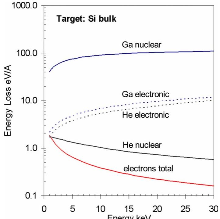
![Fic. 7. Secondary electron (SE) energy spectrum per primary electron (PE). Comparison of experimental data of Ni (Ref. 70) with the quantum mechanical electron reflection model of Schaefer and Hoelzl (Ref. 70) and the model of Chung and Everhart (Ref. 71). The surface below the experimental curve was set to the secondary electron yield=1.1 of Ni at Ey=400 eV. (b) Energy spectrum of excited surface atoms (ESA) per primary ion (PI). Monte Carlo simulation [sRIM (Ref. 73)] of the energy normal to the surface. The nonsputtered dislocated Si atoms constitute the excited surface atoms responsible for dissociation (surface below the curve, E<4.7 eV). At 30 keV, the ESA yield is Ypg,=5.5 Si/Ga ion and the sputter yield is Y;=2.6 Si/Ga ion. Besides the direct interaction with the beam, the dissocia- tion of surface adsorbed molecules involves substrate medi- Incident primary ions also incur inelastic and elastic col- lisions, which are often referred to as electronic and nuclear collisions in the FIB community. Heavier ions such as gal- lium lose a significant fraction of their energy in nuclear collisions. As a consequence they have a very short range compared to electrons (see Appendix A) and dislocate many substrate atoms along their trajectory. The dislocated atoms themselves further collide with neighboring substrate atoms in nuclear collisions and initiate collision cascades giving rise to sputtering and a distribution of excited surface atoms around the incident primary ion beam [see Fig. 6(b)]. Sec- ondary electrons are generated during inelastic collisions of primary ions. For Ga ions impinging with 1—30 keV onto](https://figures.academia-assets.com/66491804/figure_007.jpg)

![Fic. 8. MC-simulated radial distributions of emitted secondary electrons (SEs) and backscattered electrons (BSEs) per primary electron (PE): Zero diameter electron beam impinging normal with 25 and 3 keV at r=0 on planar bulk silicon. The SE exit depth was taken as 5.2 nm and the mean exit energy as 70 eV. (a) Double-log plot showing the SE distribution tails extending to the range of backscattered electrons Rgsg. (b) Log plot of the secondary electron flux. Comparison of the FWHM and FW50 (full width containing 50% secondary electrons). For both electron beam and ion beam induced processes, the minimum dimensions of the structures that can be pro- duced are larger than the incident beam diameters. The radial flux distributions of the emitted secondary and backscattered electrons and of the excited surface atoms determine the minimum dimensions of the structures that can be fabricated. Calculations of these radial distributions rely on Monte Carlo simulations. Figure 8(a) shows the radial flux distributions for electron bombardment of bulk silicon with a zero diam- eter beam. The emitted secondary electron distribution com- prises all electrons with an exit energy <50 eV and the back- scattered distribution all electrons with energies 250 eV until the incident electron energy. The MC program MOCASIM (Ref. 81) was used and works with small-angle and large-angle Mott cross sections for inelastic energy losses and with Gryzinski and Moller cross sections (inner shell excitation)®’ * for inelastic collisions. It applies a straight line approximation with exponential decrease for secondary electron generation and parametrized escape depths and exit energies.*°*’ The radial density of secondary electrons is one to two orders of magnitude larger than backscattered elec- Analogous MC simulations for excited surface atoms gen- erated by incident primary ions could be performed but we would like to mention an experimental approach to estimate the extent of this distribution proposed by Ref. 67: from measured chemical FIB deposition yields Yp [deposited metal atoms/ion], the diameter of the excited surface atom distribution is obtained by calculating how much surface the number of decomposed molecules initially covered, namely,](https://figures.academia-assets.com/66491804/figure_009.jpg)


![Fic. 11. (a) Electron impact deposition cross section of benzene [reproduced from Kunze (Ref. 110)]. For comparison the generic ionization cross sections according to Alman (Ref. 97) and the BEB theory (Ref. 96) are shown. (b) Electron impact deposition cross section for W(CO), and secondary electron (SE) yield of pure W [reproduced from Hoyle (Ref. 64)].](https://figures.academia-assets.com/66491804/figure_012.jpg)


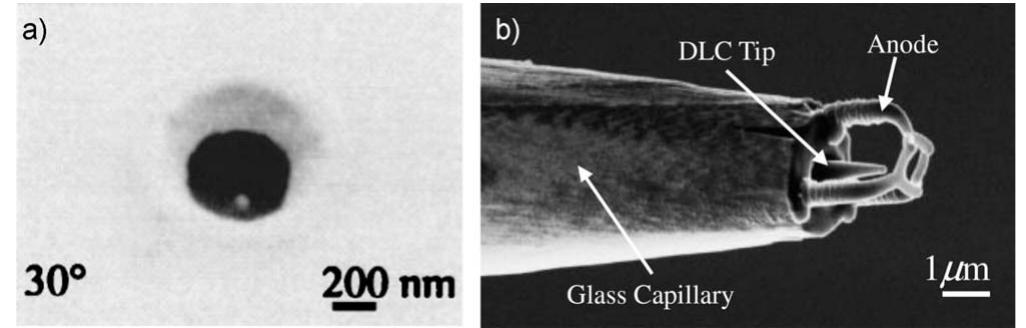
![Fic. 44. TEM of an amorphous DLC pillar showing core Ga implantation (dark grains). Deposited with phenantrene and 30 keV Ga’ ions (taken from Ref. 27). 7 The composition and microstructure of copper’ ° (see Fig. 45) and gold**° films obtained by focused ion beam induced deposition using organometallic precursors have also been studied. In the case of gold the precursor was dimethylgold hexafluroacetylacetonate, and in the case of copper it was (hfa)CuVTMS — [copper(I)-hexafluroacetylacetonate _tri- methylvinylsilane]. The films consist of either metal particles 50—100 nm diameter in a carbon matrix, or columns of](https://figures.academia-assets.com/66491804/figure_043.jpg)


![Fic. Al. Electron range R; [Eq. (A1)] and projected ranges of ions in bulk silicon according to SRIM (Ref. 73).](https://figures.academia-assets.com/66491804/figure_057.jpg)
![Fic. D2. MC simulation of dissipated energy H(z) for 3 keV electrons (Ref. 81) and 30 keV Ga and He ions [srim (Ref. 73)]. Note the differences in energy and depth for the two ion species.](https://figures.academia-assets.com/66491804/figure_059.jpg)


![“From density and molar mass [Eq. (2.8b)]. b . . Longest dimension of molecule. “Apparent diameters from Ref. 176. Note the different diameters for XeF, obtained from the different methods TABLE VI. Summary of vapor pressures (P,,,) and molecule diameters (6,,,) of selected precursors. The mean free path X was calculated at vapor pressure according to Eq. (2.8a). The monolayer density was calculated according to ny=1 15467. The Knudsen number (Kn=)/diameter) was calculated for a typical tube diameter of 0.6 mm.](https://figures.academia-assets.com/66491804/table_005.jpg)
![TABLE VII. Skirt MC simulations [Mocasim (Ref. 81)] of incident electrons (zero diameter beam, 30 and 3 keV) traversing 1 mm water vapor at a pressure of 1.4 mbar (density: 1X 10-° g/cm?). Mean free electron paths (\,), the fraction of scattered incident primary beam electrons (Ng), and skirt full widths comprising 10% and 50% of all scattered electrons are given.](https://figures.academia-assets.com/66491804/table_006.jpg)


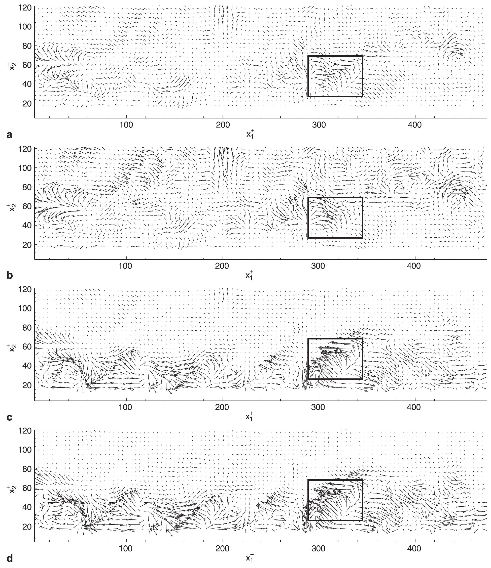
![Fig. 2a-c. Visualization of an isolated turbulent eddy by Galilean | decomposition for three different convection velocities: a ] Ug = 0.65 Ucz3 b Ue = 0.78 Uc c Ug = 0.91 Uc... Ug = 0.78 n Uc, is the ‘correct’ convection velocity based upon the Kline anc Robinson (1989) definition](https://figures.academia-assets.com/48211677/figure_002.jpg)


![From Fig. 7 it can be seen that the dimensionless mean contact pressure of the finite element analysis at w/w,=110 approaches the value p/Y =2.8. This is identical to the ratio between the hardness and yield strength found experimentally for many mate- rials as indicated by Tabor [18]. Hence, the value of p at this point is that of the material hardness, H, and, hence, w/w,=110 marks the inception of the fully plastic regime where the mean contact pressure assumes a constant value equals to the material hardness.](https://figures.academia-assets.com/50439339/figure_007.jpg)


![The most commonly used spatial correlation function shown in Table 1 is the gaussian function. It provides a very smooth and infinitely differentiable surface and is defined with only one parameter that is used to control the range of influence of nearby points. The gaussian function is a special case of the exponential function when p=2. The exponential function permits control of both the range of influence and the smoothness of the approximation function, though it is not infinitely differentiable like the gaussian function. The cubic function has only one parameter like the gaussian function and can control the range of influence but is only differentiable once. The Matern function, like the exponential function, has two parameters to control its properties. Stein [13] suggests this function is superior to the others due to its flexibility to control the selection of parameters to control its differentiability and the range of influence. In this work, the exponential spatial correlation function is used, requiring the selection of the optimal @ and p parameters.](https://figures.academia-assets.com/48908621/table_001.jpg)


