Bereits im 19. Jahrhundert formulierte John S. Mill eine einfache aber unerlässliche Voraussetzung für kausale Beziehungen: "the cause has to precede the effect in time". Für eine aufgeklärte Wissenschaft war damit der Königsweg für die...
moreBereits im 19. Jahrhundert formulierte John S. Mill eine einfache aber unerlässliche Voraussetzung für kausale Beziehungen: "the cause has to precede the effect in time". Für eine aufgeklärte Wissenschaft war damit der Königsweg für die Analyse kausaler Beziehungen vorgezeichnet, der allein dadurch beschritten w erden kann, dass im Experiment die durch einen bewusst gesetzten Stimulus behandelte Versuchgruppe eine Veränderung erfährt und sich darum -nachdem eine gewisse Zeit verstrichen ist -von der Kontrollgruppe unterscheidet. Kausale Analyse im experimentellen Design impliziert eine Längsschnittperspektive, weil Messungen der abhängigen Variable sowohl vor als auch nach Verabreichung des experimentellen Stimulus durchgeführt werden und sich bei der zweiten Messung ceteris paribus die Unterschiede zwischen den im Idealfall zufällig zusammengesetzten Gruppen logisch zwingend auf den Stimulus zurückführen lassen. So überzeugend die Rationalität der experimentellen Erkenntnismethode auch ist -in der deutschen Soziologie stellt sie eher eine Randerscheinung dar und man greift zumeist auf quasi-experimentelle Designs zurück. 1 Allerdings ermöglicht eine Längsschnittperspektive auch in diesen Studien kausale Analysen, die, wenngleich nicht ohne Theorie, wesentlich näher an der Empirie orientiert sein können, als Querschnittsanalysen. Analysen über die Zeit ermöglichen zeitveränderliche Messungen der abhängigen und unabhängigen Variablen. Auf diese Weise nähert sich die häufig auf Umfragedaten basierende Kausalanalyse dem experimentellen Design wieder an, da untersucht werden kann, inwieweit der Prozess der Veränderung der abhängigen Variable aus dem Prozess der Veränderung von unabhängigen Variablen resultiert. Daher ist es zu begrüßen, wenn in Lehrbüchern systematisch und verständlich in statistische Verfahren der Längsschnittanalyse eingeführt wird. Das im Jahre 2003 erschienene Buch "Applied longitudinal analysis" von Singer und Willet erfüllt diese Aufgabe in sehr innovativer Weise, da erstmals zwei unterschiedliche Zugänge zur Längsschnittanalyse ausführlich dargestellt und miteinander verglichen werden. Es handelt sich dabei einerseits um Messwiederholungsmodelle, die als "multilevel model for change" bezeichnet werden, andererseits um Hazardmodelle für diskrete und stetige Zeit, in der deutschsprachigen Soziologie eher bekannt unter der Bezeichnung "Ereignisanalyse". Im Prinzip ist ein derartiges Lehrbuch schon lange überfällig, da die beiden methodischen Ansätze des Messwiederholungsdesigns (auch bekannt als Panelanalyse) und der Ereignisanalyse zumeist in unterschiedlichen Forschungszweigen Anwendung finden und leider manchmal Unkenntnis herrscht über die Angemessenheit oder über mögliche Vorteile des jeweils anderen methodischen Zugangs. 1 Vgl. zu sozialwissenschaftlichen und medizinischen Experimenten insbesondere David M. : Design and Analysis of group randomized trials. Oxford: University Press.


![ORDINARY LEAST SQuARES (36)* *Dependent variable p = log(P} — log(P_|) where P is quarterly U.K. consumer price index. w = lagt W) where H/ is the U.K. index of manual wage rates. Sample period 1958-[] to 1977-IL. TABLE I The least squares estimates of this model are given in Table L. The fit is quite good, with less than | per cent standard error of forecast, and all ¢ statistics greater than 3. Notice that p_, and j_, have equal and opposite signs, suggesting that it is the acceleration of inflation one year ago which explains much of the short-run behavior in prices.](https://figures.academia-assets.com/5948763/table_001.jpg)


![The third element of A~'f is the limit random variable for n(6, — 1) given in Dickey and Fuller [7]. Using the fact that S2 converges in probability to o?, we obtain](https://figures.academia-assets.com/43130769/figure_004.jpg)


![This function also implausibly implies, as Pratt [17] and Arrow [1] have noted, that the insurance premiums which peo- ple would be willing to pay to hedge given risks rise progress- ively with wealth or income. For a related result, see Hicks (6, p. 802]. gs It is, consequently, very relevant to note that by using the Bienaymé-Tchebycheff inequality, Roy [19] has shown that investors operating on his “Safety First” principle (i.e. make risky in- vestments so as to minimize the upper bound of the probability that the realized outcome will fall below a pre-assigned “disaster level’) should maximize the ratio of the excess expected port- folio return (over the disaster level) to the standard deviation of the return on the port- folio?! — which is precisely our criterion of max 6 when his disaster level is equated to the risk- free rate r*. This result, of course, does not depend on multivariate normality, and uses a different argument and form of utility function. ML. Ci pee ntinea Mhaneneee nerdy 24n Onreweurlanwnn](https://figures.academia-assets.com/30555591/figure_001.jpg)
![The conclusions stated in the text are obvious from the graph of this case (which incidentally is formally identical to Hirschleifer’s treatment of the same case under certainty in [¥].)](https://figures.academia-assets.com/30555591/figure_002.jpg)


![t = 1951:II to 1984: IV. Numerical maximization of the conditional log likeli- hood function led to the maximum likelihood estimates reported in Table I. Also reported are asymptotic standard errors.’ MAXIMUM LIKELIHOOD ESTIMATES OF PARAMETERS AND ASYMPTOTIC STANDARD ERRORS BASED ON Data FOR U.S. REAL GNP, ¢ = 1952: II To 1984: IV hood function led to the maximum hkelinood estimates reported in iable 1. Also reported are asymptotic standard errors.’ One possible outcome that might have been expected a priori would associate the states s,=0 and 1 with slow and fast growth rates for the U.S. economy, corresponding to decade-long changes in trends. In fact, however, the sample likelihood is maximized by a negative growth rate of —0.4% per quarter during state 0 and a positive growth of (a) + a,) = +1.2% during state 1. These values clearly correspond to the dynamics of business cycles as opposed to long-term variations in secular growth rates. Indeed, the first- and second-order serial correlation in logarithmic changes of real GNP seem to be better captured by shifts between states rather than by the leading autoregressive coefficients, as indicated by the fact that ¢, and 5 come out remarkably close to zero. Negative coefficients at lags 3 and 4 suggest the possibility that the method used by the Bureau of Economic Analysis for deseasonalizing introduces spurious periodicity when applied to data generated by a nonlinear process such as this one. These coefficients further suggest that investigating a higher-order Markov process for the trend might also be a fruitful topic for future research. Figure 1 reports the estimated probability that the economy is in the negative growth state (P[S, = 0]) based on currently available information (panel A) and fo eee ee Se : E Ok SS (eae em oe ees Me Pe Se a, Se rs Sere arent TABLE I](https://figures.academia-assets.com/4682898/table_001.jpg)


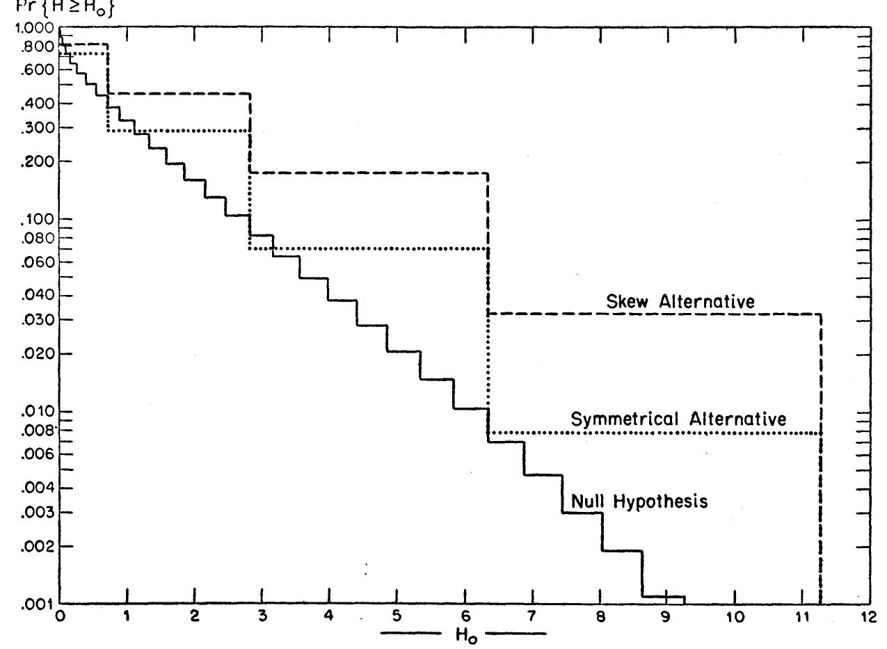


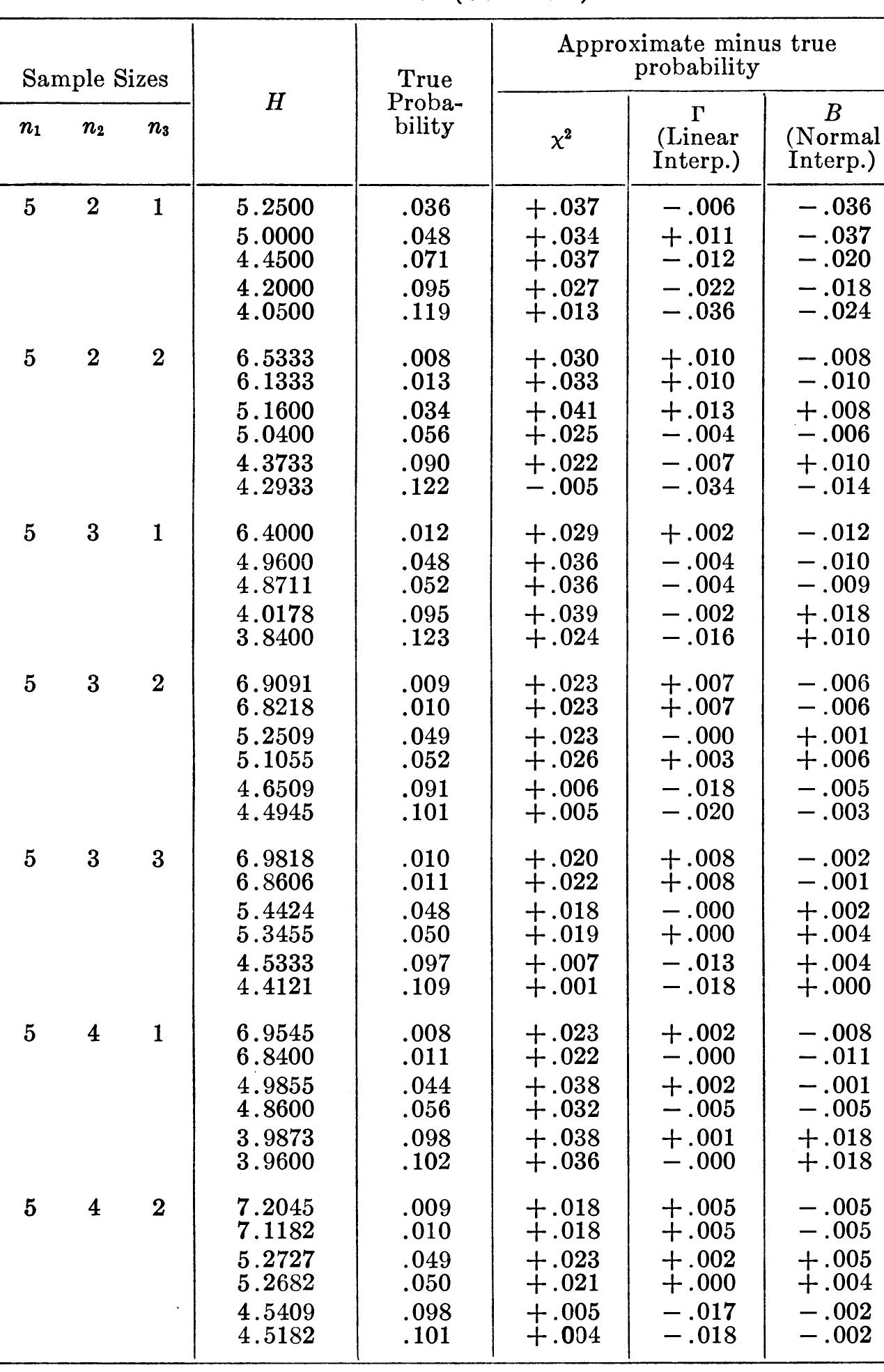
![BROWNLEE EXAMPLE [2, p. 36] 10 Pitman [41] gives a test which is like H except thatit considers possible permutations of the actual observations instead of their ranks. For the example of Table 3.1, Pitman’s test yields a two-tail prob- ability of 5/126 or 0.03968.](https://figures.academia-assets.com/12098243/table_001.jpg)


![tain spatial position. The next decisions are the position of the first collision and the nature of that collision. If it is deter- mined that a fission occurs, the number of emerging neutrons must be decided upon, and each of these neutrons is eventually followed in the same fashion as the first. If the collision is decreed to be a scatter- ing, appropriate statistics are invoked to determine the new momentum of the neu- of integers whose properties have been extensively studied. Clearly, this chain of numbers repeats after some point. H. Lehmer has suggested a scheme based on the Kronecker-Wey] theorem that gener- ates all possible numbers of n digits be- fore it repeats. (See “Random-Number Generators” for a discussion of various approaches to the generation of random numbers.) contributed much to its development, in- cluding its application during the war to neutron multiplication in fission devices. For a long time his collection of research interests included pattern development in two-dimensional games played according to very simple rules. Such work has lately emerged as a cottage industry known as cellular automata. tron. When the neutron crosses a material boundary, the parameters and characteris- tics of the new medium are taken into ac- count. Thus, a genealogical history of an individual neutron is developed. The pro- cess is repeated for other neutrons until a statistically valid picture is generated.](https://figures.academia-assets.com/6356196/figure_003.jpg)


![AMERICAN STATISTICAL ASSOCIATION JOURNAL, JUNE 1962 The unit and zero matrices in (4.5) are of order /X/. Thus there are g=(M—1)1 restrictions, as stated above. Roy’s [10, p. 82] very elegant derivation of this test does not involve the likelihood-ratio approach. However, as shown in a straight-forward manner in Appendix A, the likelihood-ratio approach leads to the same test statistic. If the disturbance covariance matrix were known (4.4) would give an exact test of the hypothesis in (4.1). When an estimate of this matrix is employed in constructing the test statistic, we show in Appendix B that the resulting statistic, say F, is equal to the statistic in (4.4) plus an error which is 0(n-¥/?) in probability. Then by a theorem in [5, p. 254], F will have the same asymptotic distribution as Fy,-m. But, as shown in Appendix A, —2 log X=qFgn-m+0(n—) where d is the likelihood ratio for testing the hypothesis in (4.1). It is known [8, p. 259 and 12, p. 151] that —2 log , and thus gFgn-m (and qgF), is asymptotically distributed as x{=x{y-y1, where 1(M —1) is the number of restrictions involved in (4.1). For small samples there is some question about how to proceed. We can compute gf and use gf’s asymptotic distribution, x7, assuming that the asymp- totic results apply. Another alternative, which may be better, would be to as- sume that F’s distribution is closely approximated by that of Fg,n—m.7](https://figures.academia-assets.com/32800771/figure_005.jpg)


![Size and power of unit root tests in heterogeneous panels. Experiment 1: No serial correlation, no time trend Notes: This table reports the size and power of the t-bar test statistic Zjpq- defined by (3.13) and the Levin and Lin (ZL) test, respectively. The underlying data is generated by yi =(1—@) wit byir—-1 +60, i= 1,...,N, t= —51, —50,...,7, where we generate yw; ~ N(0,1) and é ~ N(0, a7) with oF ~ U[0.5, 1.5]. Mi and oF are generated once and then fixed in all replications. The test statistics are obtained using the DF regressions: Ay =a + Biyi2—1 +6, t=1,2,...,7, i=1,2,...,N. The size (P=1) and power (@ =0.9) of the tests are computed at the five percent nominal level. Number of replications is set to 2,000. The result for N = 1 is reported for comparison, and DF refers to the Dicky—Fuller test. The LZ test for T = 10 is not included, since the adjustment factors necessary for computing the LL statistic are not reported in Levin and Lin (1993). Table 4](https://figures.academia-assets.com/46981058/table_007.jpg)
![Notes: The results in this table are computed using the same data generating process as in Table 4 except that ¢;;’s now follow the AR(1) processes: éj = pjé,;—-1 +e, t=1,...,T, i=1,...,N, where e; ~ N(0, oH and p; ~ U[0.2,0.4]. p;’s are generated once and then fixed in all replications. The reported size and power of the tests are based on the individual ADF regressions: A yj = a + Bi ¥i2—1 + Vy pPiAAVir—j + et, t= 1,...,7, i=1,...,N. The test statistic Wig, is defined in (4.10). See also the notes to Table 4. Size and power of unit root tests in heterogeneous panels. Experiment 2: AR(1) Errors with p; ~ U[0.2, 0.4], No Time Trend](https://figures.academia-assets.com/46981058/table_008.jpg)
![Notes: The results in this table are computed using the same data generation process as in Table 4 except that ¢;’s now follow the MA(1) processes, & =e + Weir—1, t=1,...,7, i=1,...,N, where ej ~ N(0, a? and yj ~ U[ — 0.4, —0.2]. y’s are generated once and then fixed in all replications. See also the notes to Tables 4 and 5. Size and power of unit root tests in heterogeneous panels. Experiment 3: MA(1) errors with yj ~ U[ — 0.4, —0.2], no time trend](https://figures.academia-assets.com/46981058/table_009.jpg)
![Notes: The results in this table are computed using the same data generating process as in Table 5. But, the reported size and power of the tests are now based on the individual ADF regressions with time trend included: Ay = aj + Oj + Bivix—1 + ae pi AVir—j + en, t=1,...,T, i=1,...,N. See also the notes to Tables 4 and 5. Size and power of unit root tests in heterogeneous panels. Experiment 4: time trend, AR(1) errors with pi ~ U[0.2, 0.4]](https://figures.academia-assets.com/46981058/table_010.jpg)


![Table II. Equilibrium correction form of the ARDL(6, 0, 5, 4, 5)
earnings equation
Notes: The regression is based on the conditional ECM given by (30)
using an ARDL(6, 0,5, 4,5) specification with dependent variable, Aw;
estimated over 1972ql-— 199744, and the equilibrium correction term
H%-1 is given in (31). R is the adjusted squared multiple correlation
coefficient, G is the standard error of the regression, AI and Bae are
Akaike’s and Schwarz’s Bayesian Information Criteria, xXbc (4), XF 2 (1),
x7 (2), and x20) denote chi-squared statistics to test for no residual
serial correlation, no functional form mis-specification, normal errors and
homoscedasticity respectively with p-values given in [-]. For details of
these diagnostic tests see Pesaran and Pesaran (1997, Ch. 18).](https://figures.academia-assets.com/46980930/table_011.jpg)


![Size of 7, and 4,, 5% level, iid errors. integer[12(7./100)'/*]. These choices of / follow Schwert (1989) and other recent simulations.](https://figures.academia-assets.com/46980886/table_001.jpg)


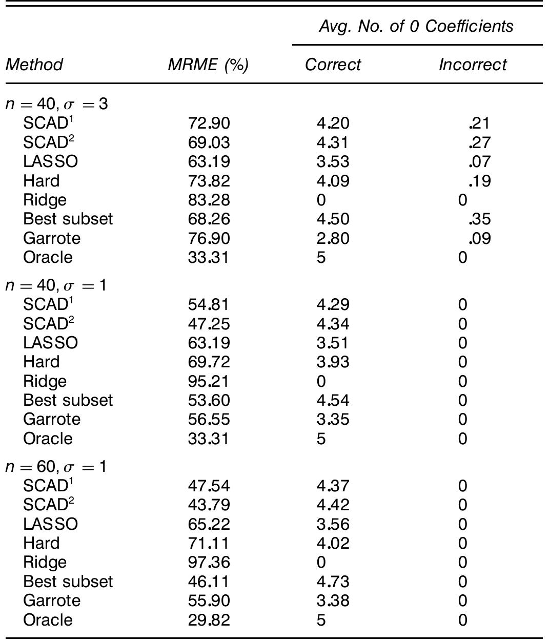
![Figure 4. Plot of p\\(@) Functions Over @ > 0 (a) for L, Penalties, (b) the Hard Thresholding Penalty, and (c) the SCAD Penalty. In (a), the heavy le corresponds to L,, the dash-dot line corresponds to L.;, and the thin line corresponds to L, penalties. [see Fig. 2(c)]. This solution is owing to Fan (1997), who gave a brief discussion in the settings of wavelets. In this article, we use it to develop an effective variable selection procedure for a broad class of models, including linear regression models and generalized linear models. For simplicity of presentation, we use the acronym SCAD for all procedures using the SCAD penalty. The performance of SCAD is similar to that of firm shrinkage proposed by Gao and Bruce (1997) when design matrices are orthonormal. We now compare the performance of the four previously stated thresholding rules. Marron, Adak, Johnstone, Neumann, and Patil (1998) applied the tool of risk analysis to under- stand the small sample behavior of the hard and so olding rules. The closed forms for the L, risk R(6, 0) = E(@ — 0)? were derived under the Gaussian model Z ~N(0,q@7) for hard and soft threshold and Johnstone (1994b). The risk function of the SCA t thresh- unctions ing rules by Donoho D thresh- olding rule can be found in Li (2000). To gauge the perfor- mance of the four thresholding rules, Figure 5(c) depicts their L, risk functions under the Gaussian model Z ~ N(@, 1). To make the scale of the thresholding parameters roughly com- parable, we took A = 2 for the hard thresholding rule and adjusted the values of A for the other thresholding rules so that their estimated values are the same when 6 = 3. The SCAD](https://figures.academia-assets.com/31172723/figure_003.jpg)