César Osses Espinoza
580 California St., Suite 400
San Francisco, CA, 94104
The paper presents an in-depth analysis of the seismic behavior of structures, focusing on the fundamental principles of plate tectonics as a precursor to understanding earthquake mechanics. It discusses the mechanisms of seismic wave propagation, interplate and intraplate earthquake occurrences, and the relevant factors influencing structural response during seismic events. Through a mix of theoretical modeling and empirical data, the research highlights the need for effective damping strategies and response analysis to improve earthquake resilience in engineered structures.
![Figure 1.1 Inside the earth (Source: Murty, C.V.R. “IITK-BMPTC Earthquake Tips.” Public domain, National Information Centre of Earthquake Engineering. 2005. http://nicee.org/EQTips.php - accessed April 16, 2009.) the inner core, the outer core, the mantle, and the crust, as shown in Figure 1.1. The upper-most layer, called the crust, is of varying thickness, from 5 to 40 km. The discontinuity between the crust and the next layer, the mantle, was first discovered by Mohorovi¢i¢ through observing a sharp change in the velocity of seismic waves passing from the mantle to the crust. This discontinuity is thus known as the Mohorovici¢ discontinuity (““M discontinuity”). The average seismic wave velocity (P wave) within the crust ranges from 4 to 8kms'. The oceanic crust is relatively thin (S—15 km), while the crust beneath mountains is relatively thick. This observation also demonstrates the principle of isostasy, which states that the crust is floating on the mantle. Based on this principle, the mantle is considered to consist of an upper layer that is fairly rigid, as the crust is. The upper layer along with the crust, of thickness ~120 km, is known as the lithosphere. Immediately below this is a zone called the asthenosphere, which extends for another 200 km. This zone is thought to be of molten rock and is highly plastic in character. The asthenosphere is only a small fraction of the total thickness of the mantle (~2900 km), but because of its plastic character it supports the lithosphere floating above it. Towards the bottom of the mantle (1000-2900 km), the variation of the seismic wave velocity is much less, indicating that the mass there is nearly homogeneous. The floating lithosphere does not move as a single unit but as a cluster of a number of plates of various sizes. The movement in the various plates is different both in magnitude and direction. This differential movement of the plates provides the basis of the foundation of the theory of tectonic earthquake. Below the mantle is the central core. Wichert [1] first suggested the presence of the central core. Later,](https://figures.academia-assets.com/31938309/figure_001.jpg)


![Table 1.1 Frequency of occurrence of earthquakes (based on observations since 1900) 1.3.5 Energy Release Newmark and Rosenblueth [9] compared the energy released by an earthquake with that of a nuclear explosion. A nuclear explosion of 1 megaton releases 5 x 10'°J. According to Equation 1.12, an earthquake of magnitude Ms = 7.3 would release the equivalent amount of energy as a nuclear explosion of 50 megatons. A simple calculation shows that an earthquake of magnitude 7.2 produces ten times more ground motion than a magnitude 6.2 earthquake, but releases about 32 times more energy. The E of a magnitude 8.0 earthquake will be nearly 1000 times the E of a magnitude 6.0 earthquake. This explains why big earthquakes are so much more devastating than small ones. The amplitude numbers are easier to explain, and are more often used in the literature, but it is the energy that does the damage. The length of the earthquake fault L in kilometers is related to the magnitude [10] by](https://figures.academia-assets.com/31938309/table_001.jpg)
![Table 1.2 Modified Mercalli intensity (MMI) scale (abbreviated version) Although the subjective measure of earthquake seems undesirable, subjective intensity scales have played important roles in measuring earthquakes throughout history and in areas where no strong motion instruments are installed. There have been attempts to correlate the intensity of earthquakes with instrumentally measured ground motion from observed data and the magnitude of an earthquake. An empirical relationship between the intensity and magnitude of an earthquake, as proposed by Gutenberg and Richter [6], is given as The last one, which has ten grades, 1s still used 1n some parts of Europe. The Mercalli-Cancani—Sieberg scale, developed from the Mercalli (1902) and Cancani (1904) scales, is still widely used in Western Europe. A modified Mercalli scale having 12 grades (a modification of the Mercalli-Cancani—Sieberg scale proposed by Neuman, 1931) is now widely used in most parts of the world. The 12-grade Medved— Sponheuer—Karnik (MSK) scale (1964) was an attempt to unify intensity scales internationally and with the 8-grade intensity scale used in Japan. The subjective nature of the modified Mercalli scale is depicted in Table 1.2.](https://figures.academia-assets.com/31938309/table_002.jpg)


![Figure 2.9 Variation of rms value of acceleration with time for uniformly modulated non-stationary process Records of actual strong motion time history show that modeling of an earthquake process as a stationary random process is not well justified as the ensemble mean square value varies with time. The mean square value gradually increases to a peak value, remains uniform over some time, and then decreases as shown in Figure 2.9. Such type of behavior is often modeled as a uniformly modulated non- stationary process [3]. Such a process is represented by an evolutionary power spectral density function. The evolutionary spectrum is obtained by multiplying a constant spectrum with a modulating function of time ¢ and is given as:](https://figures.academia-assets.com/31938309/figure_040.jpg)


![Figure 2.50 Exponential type modulating function in which Ag is the scaling factor and f,, f2, and f3 are the transition times of the modulating function. A modified form of the trapezoidal type modulating function [29] is shown in Figure 2.49 and is given by](https://figures.academia-assets.com/31938309/figure_086.jpg)


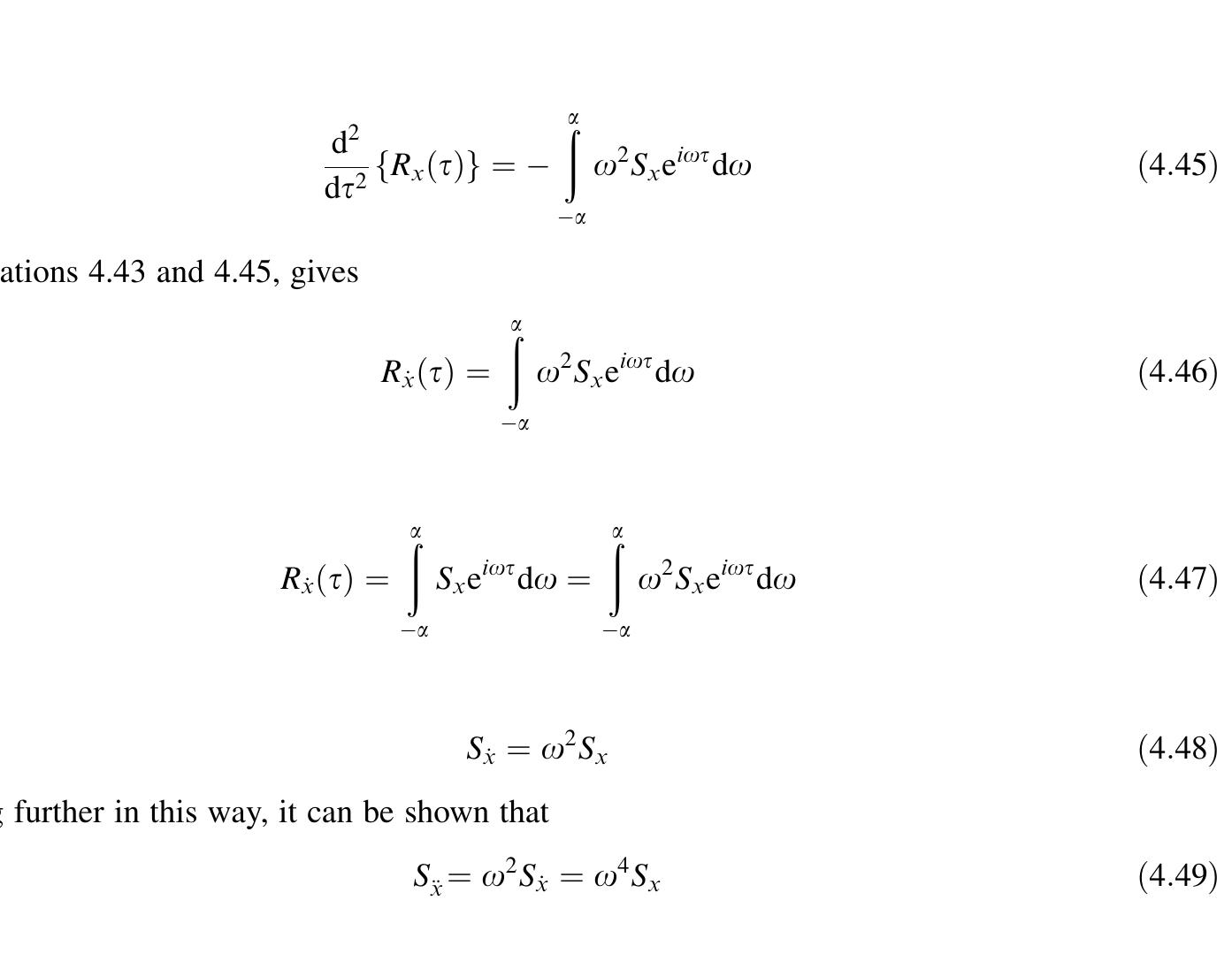
![Figure 4.4 Shaded area at frequency w contributing to the mean square value in which r? is the mean square value of the process; E[ ] indicates the expected value, that is, the average or mean value. Equation 4.26a provides a physical meaning of the power spectral density function. The area under the curve of the power spectral density function is equal to the mean square value of the process. In other words, the power spectral density function may be defined as the frequency distribution of the mean square value. At any frequency o, the shaded area as shown in Figure 4.4 is the contribution of that frequency to the mean square value. If the square of x(t) is considered to be proportional to the energy of the process [as in E(t) =!4Kx(t)*], then the power spectral density function of a stationary random process in a way denotes the distribution of the energy of the process with frequency. For random vibration analysis of structures in the frequency domain, the power spectral density function (PSDF) forms an ideal input because of two reasons:](https://figures.academia-assets.com/31938309/figure_153.jpg)


![Figure 5.2 Variation of correlation coefficient p;; with the modal frequency ratio «; /;; abscissa scale is logarithmic pj May be ignored as it is assumed in the SRSS combination rule. SRSS and CQC rules for the combination of peak modal responses are best derived assuming a future earthquake to be a stationary random process (Chapter 4). As both the design response spectrum and power spectral density function (PSDF) of an earthquake represent the frequency contents of ground motion, a relationship exists between the two. This relationship is investigated for the smoothed curves representing the two, which show the averaged characteristics of many ground motions. If the ground motion is assumed to be a stationary random process, then the generalized coordinate in each mode of vibration is also a random process. Therefore, there a cross correlation (represented by cross PSDF) between the generalized coordinates of any two modes is present. Because of this, it is reasonable to assume that a correlation coefficient p,; exists between the two modal peak responses. Derivation of p, (Equation 5.15) as given by Der Kiureghian [2] is based on the above concept. There have heen ceveral attemnte to ectahlich 9a relatinnchin hetween the PSDE and the recnonce](https://figures.academia-assets.com/31938309/figure_175.jpg)


![The analysis replaces the soil by spring—dashpots as shown in Figure 7.55. The spring stiffness and damping coefficients of the dashpots are derived by combining Mindlin’s static analysis of the soil pressure at a depth within the soil and the soil impedance functions. The details of the derivation are given in references [12, 13]. The stiffness and damping coefficients of the matrices corresponding to the DOF are coupled unlike the condition of Winkler’s bed. However, a simplified analysis can be performed by ignoring the off-diagonal terms and by using the diagonal terms to assign stiffness and](https://figures.academia-assets.com/31938309/figure_288.jpg)


![een gn ne nnn en een ene en nen ee enn ne ne eee nn eee nn een ee nee enn nee ee ee OE The pipeline is also subjected to axial vibration along the length of the pipe due to P waves traveling along the pipeline. Analysis as described above can be carried out for axial vibration of the pipeline, with the soil being replaced by equivalent springs and dashpots. The stiffness and damping coefficients of the springs and dashpots are similarly obtained as for the case of transverse oscillation. For a simplified analysis, stiffness and damping coefficients of the springs and dashpots may be obtained by ignoring the off-diagonal terms of the soil stiffness and damping matrices. Figure 7.56 provides the frequency independent stiffness and damping coefficients of the equivalent springs and dashpots for transverse and axial vibrations of buried pipelines [12]. These coefficients may be used to obtain the stiffness and damping coefficients as follows: Figure 7.56 Variation of frequency independent spring and damper coefficients with d/r](https://figures.academia-assets.com/31938309/figure_291.jpg)

![Stiffness matrix for the structure corresponding to the DOF, shown in Figure 7.57, is obtained as: [K;], is added to the K part of the [K], matrix and then rotational degrees of freedom are condensed out. The resulting stiffness matrix is the soil—pipe stiffness matrix. For axial vibration, [K,],, is directly added to [K],,- To construct the damping matrix, [K], is condensed to eliminate 6 degrees of freedom. Assuming Rayleigh damping, [C], for the pipe is obtained using the first two frequencies of the soil—-pipe system. Note that the eigen value problem cannot be solved without adding spring stiffness to the pipe stiffness matrix. [C,], is added to [C], to obtain the damping matrix of the soil—-pipe system. In a similar way, a damping matrix for the axial vibration can be determined. Results of the computation are given below. The first two frequencies of the soil—pipe system and « and f values are:](https://figures.academia-assets.com/31938309/figure_293.jpg)


![Figure 8.3. Hasofer—Lind reliability index with linear performance function When the limit state function is non-linear, the computation of the minimum distance becomes an optimization problem, that is, Shinozuka [4] obtained an expression for the minimum distance as:](https://figures.academia-assets.com/31938309/figure_296.jpg)


![In the above problem, if material uncertainty is included then the limit state function takes the form where Lo is the probability of starting below the threshold, « is the decay rate, and T is the duration of the process. At high barrier levels, Lo is practically one and the decay rate is given by the following expressions with double barrier (ap) and one sided barrier (~s) respectively [12],](https://figures.academia-assets.com/31938309/figure_307.jpg)


![Figure 9.44 A model of Teflon coated viscoelastic damper where C|.] and DJ[.] are linear differential operators with constant coefficients. Using a Laplace transformation, Equation 9.78 provides a transfer function H(s) in the form of](https://figures.academia-assets.com/31938309/figure_360.jpg)


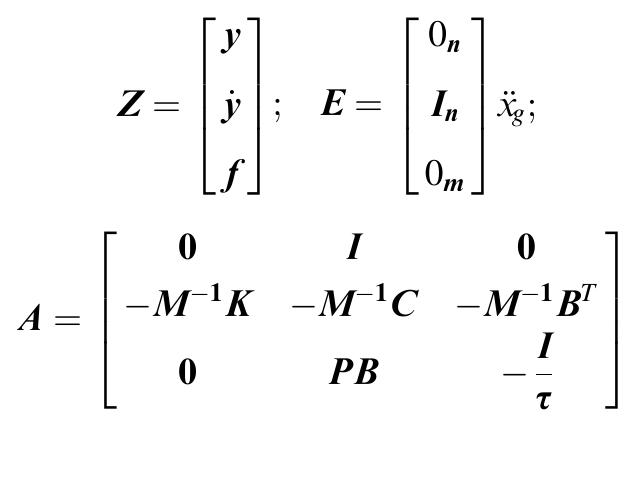


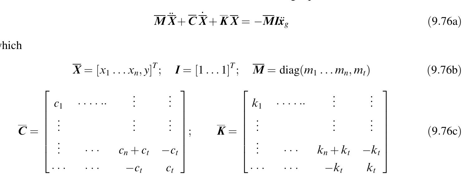
![regulator (LQR) control, pole placement technique, instantaneous optimal control, discrete time control, sliding mode control, independent modal space control, bounded state control, predictive control, H, control, and so on [11,12]. The control mechanisms, which have been developed and used in experiments and in practice, include actuated mass damper (AMD), actuated tuned mass damper (ATMD), active tendon system (AT), and so on (Figure 9.53). Active control algorithms generate the required control signal that drives the actuators of the control device. Before describing the control algorithms, it is desirable to understand the effect of control forces on the response of a structure under ideal conditions. Consider the equation of motion of a multi-degrees of freedom system under a set of control forces u:](https://figures.academia-assets.com/31938309/figure_369.jpg)

![in which e = X—X. Equation 9.144 is similar to Equation 9.136a. For complete state controllability, that is, |A—K-.C] to be a state matrix, [A—K.C] has arbitrarily desired eigen values. Thus, K, can be designed to yield the desired eigen values. The problem is similar to finding the gain matrix G for the pole placement technique (discussed later) and can be solved by Ackerman’s formula [13]. Using Ackerman’s formula, the gain matrix K, can be obtained as:](https://figures.academia-assets.com/31938309/figure_371.jpg)
![MATLAB computation to find the K, is explained with the following example. in which e = x,—Xp; Xp is the estimated state of the un-measured variables. K, as before can be obtained using Ackerman’s formula and is given by [13]: Example 9.7](https://figures.academia-assets.com/31938309/figure_372.jpg)


![For a control system described by Equation 9.149, obtain the G matrix using MATLAB for the following values of A, B, and J [13]. Note that the output matrix, that is, K of MATLAB is the G matrix. As a result, both K and G are used to denote the same gain matrix. Example 9.8A](https://figures.academia-assets.com/31938309/figure_375.jpg)