Hydraulic jump is a phenomenon caused by change in flow from super-critical to sub-critical flow with considerable energy dissipation and rise in depth of flow. This paper presents the results of experimental investigations to control the...
moreHydraulic jump is a phenomenon caused by change in flow from super-critical to sub-critical flow with considerable energy dissipation and rise in depth of flow. This paper presents the results of experimental investigations to control the hydraulic jump by providing the abrupt rise (hump) at the bed of rectangular open channel. Various types of humps were designed and fabricated based on the critical velocity analysis for the maximum discharge in the flume. These humps were placed in flume at different positions from the upstream gate to control the hydraulic jump at the downstream. From the experimental results a new relationship is proposed to control the hydraulic jump at a specified location using the hump in the bed. This gives the economical solution in agricultural field which is one of the major contributions towards the society as well as it also gives technical inputs to the researchers in the field of same research. I. INTRODUCTION A hydraulic jump is a phenomenon which has extensively been studied in the field of hydraulic engineering due to its frequent occurrence in open channel flow such as rivers and spillways. When the rapid change in the depth of flow from a low stage to high stage, the result is usually in the form of an abrupt rise at water surface, this local phenomenon is known as Hydraulic jump. By utilizing characteristics, hydraulic jump is immensely used as an energy dissipater to dissipate the excess energy of flowing water at the downstream of hydraulic structures such as spillways and sluice gates, to recover head or rise the in water level on the downstream side and thus maintain high water level in the channel for irrigation or other water distribution purposes. It is useful for increasing weight on an apron to reduce the uplift pressure under a masonry structure by raising the water depth on the apron, to increase the discharge of a sluice by holding back the tail water, to indicate special conditions of supercritical flow and of control section to decide the perfect location of gauging station, for mixing of chemicals, to remove air pockets from water supply line and to prevent water locking etc. Due to these many practical applications, hydraulic jump is an interesting topic that has caught the imagination of many researchersin 18 th century who had done the first experimental investigation of jump to till date. But the control of the jump and its location to serve all these above mentioned uses is the foremost important task for the investigators. The hydraulic jump can be controlled or affected by the number of appurtenances as baffle blocks, sills, weirs, abrupt rise and drop in the channels. As the flow in the vicinity of these appurtenances is rapidly varied, the velocity distribution is not uniform. And it is difficult to apply the momentum equation to analyze accurately the formation of jump only by means of theoretical basis; therefore for useful design information one has to rely on the experimental investigations [1]. The researchers had done laboratory experiments to develop empirical relations for universal applications and model studies were conducted for specific projects. In the 20 th century,many researchershave done experiments on hydraulic jump, amongst them one has done model study with dual spillway [2], one of them had thrown a light on the impact of hydraulic jump [3] and few from the current era; in 2005 one had studied the jump on rough bed [4], in 2011 researcher noticed


![As of June 2011, there were 15,988 desalination plants world- wide which combined produce a total of 65.2 million m? of fresh- water equivalent to 17.5 billion US gallons in over 150 countries supporting 300 million people [129]. Out of these desalination plants, reverse osmosis with about 60% share currently dominates the other desalination technologies | 133] (Fig. 2a) and this trend is expected to continue into the future followed by well-established MSF technology (26.8%) and MED technology (8%) with the remaining 5% taken by electrodialysis and other hybrid technolo- gies. Sixty percent of the desalination plants process seawater to produce freshwater (Fig. 2b) followed by brackish water (21.5%), river water (8.3%), wastewater recovery/reuse (5.7%) and other water sources (4.5%) [130]. Energy requirements for desalination technologies vary significantly in quantity and quality. Table 1](https://figures.academia-assets.com/34338939/figure_004.jpg)


![3.2.4.2. Thermal energy storage in solar desalination. Storage volume is critical to the performance of the TES tank. In desalination appli- cation powered by solar collectors, a TES tank is required to miti- gate the effects of cloudy hours and non-sunlight hours. In a recent study, the effect of TES tank volume was simulated for a low temperature desalination process (at a capacity of 100 L/d) supported by solar collectors [7]. Temperature profiles over a week of operation for the TES tank at two different volumes (1 m? and 6 m?) are shown in Fig. 8. As expected, the TES temperature pro- files followed the sinusoidal nature of the solar irradiation and the ambient temperature. Smaller TES volume (1 m?) temperatures were more responsive to these variations than higher TES volume Fig. 7. Effect of LCZ depth on the storage medium temperature profiles.](https://figures.academia-assets.com/34338939/figure_008.jpg)


![Fig. 1. A standard [10] tensile V-notch (TVN) sample made of AISI 4340 steel heat treated to 50-53 Rc](https://figures.academia-assets.com/53459721/figure_001.jpg)


![Fig. 2. Change of the y,¢9, with time. P=120 bars, T=27°C and [NaCl] = 5000 ppm.](https://figures.academia-assets.com/53085807/figure_002.jpg)


![Fig. 6. Surface tension of brine as a function of the molal concentration of NaCl [26].](https://figures.academia-assets.com/53085807/figure_006.jpg)


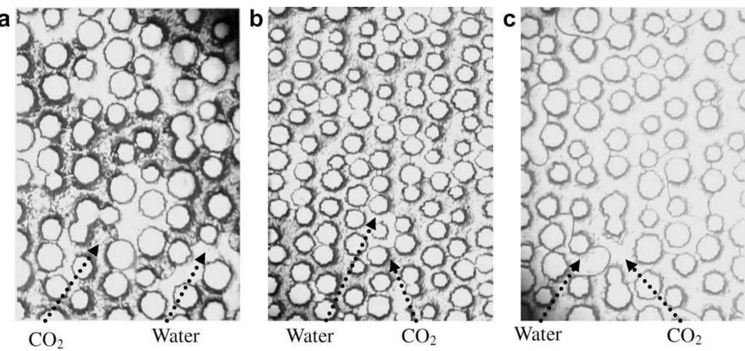
![Fig. 11. Gaseous CO (P=5 bars, T = 20 °C): (a) water-wet micromodel; (b) intermediate-wet. For water-wet micromodels and low pressures (gaseous CO;), we have observed very thin water films surrounding the solid sur- face (Figs. 11 and 12a). At higher pressures (Fig. 12b and c), we cannot observe such films. Roughness could affect the observation of these films. However, it is important to note that the same micromodel was used in these three experiments. The evolution of the film thickness is directly related to the relative affinity be- tween water, CO2 and the solid substrate. The estimation of this affinity is not straightforward since it requires many physico- chemical parameters to be taken into account, most of them not being available in the literature. Chiquet et al.’s work [30] pre- sented in the Introduction could contribute to explaining this thickness reduction. The authors attribute this behavior to a reduc- tion in electrostatic interaction that tends to stabilize the water films. Despite this behavior, the shape of the interfaces (Fig. 12)](https://figures.academia-assets.com/53085807/figure_011.jpg)


![Fig. 5. Time variation of pressure coefficients. the air barrier is smooth compared to that across the panel. Consequently, the higher-frequency pressure fluctuations have been transferred to the rainscreen. Extensive analysis of the field data in the frequency domain has been recently presented in Ref. [12]. For simplicity, only the pressure coefficients applicable to the panel and rainscreen are discussed; one of the intentions of pressure equalization to reduce pressure load on the rainscreen is another good reason for presenting results in this format.](https://figures.academia-assets.com/66590541/figure_006.jpg)


![Note: ,=porosity of rainscreen, ; =effective porosity of air barrier estimated based on orifice plate- meter equation [10]. Comparison of full-scale measurements with the provisions in ENV 1991-2-4 for rainscreen walls with permeable air barrier](https://figures.academia-assets.com/66590541/table_002.jpg)


![In the present study experiments were performed on a horizontal rectangular channel of imensions 5m X 0.25m X 0.076m in Fluid Mechanics Laboratory of Civil Department of ‘ishwakarma Institutes of Information Technology, Pune. Initially flume was set to carry the maximum discharge (Qmax=0.00195m?3/sec) for which critical velocity is calculated V.-=0.385m2/sec). On the basis of these values dimensional limits were decided for the humps and umps of different dimensions were designed and fabricated (Table no. 1) considering the specific nergy graph [9]. A series of experiments performed at different values of discharge and hydraulic imp was formed by using various humps at different locations. For each experiment initial depth, riddle depth, final depth, length of hydraulic jump, location of hump and location of hydraulic jump vere measured. The above steps were performed sequentially at different discharge. The discharge 1 the channel is measured using discharge measuring water tank. The depths were measured using oint gauge and length by using measuring scale. From the above measured quantities, velocity efore and after the jump, energy dissipation after the jump and Froude number were calculated. The tatistical analysis of position of hump with respect to the location of jump is done as the main aim f the present study. Along with this the characteristics behavior of the jump with respect to the osition of humps is also studied from the experimental observations. HI. EXPERIMENTAL OBSERVATIONS](https://figures.academia-assets.com/47350626/figure_001.jpg)


![Figure 1. Flowchart of dependencies between data sources and computation of the water scarcity index. Sources indicated in the flowchart are as follows: 1, Lehner and Doll [2004]; 2, International Commission on Large Dams [2003]; 3, World Water Assessment Programme (WWDR-II, http:/Avwdrii.sr-unh.edu/); 4, Mitchell and Jones [2005]; 5, Kallberg et al. [2005]; 6, New et al. [1999]; 7, Siebert and Doll [2008]; 8, Portmann et al. [2008]; 9, EROS, USGS (Global land cover characteristics data base, version 2.0, http:// edcdaac.usgs.gov/glec/globedoc2_0.html); 10, Food and Agriculture Organization of the United Nations (http://www. fao.org/ag/AGA info/resources/en/glw/GLW_dens.html) and Environmental Research Group Oxford (http://ergodd.zoo.ox.ac.uk/); 11, MLIT [2007]; 12, World Bank [2006, 2007; country classification, http://web.worldbank.org]; 13, FAO AQUASTAT database (http://www. fao.org/nr/water/aquastat/data/); 14, International Groundwater Resources Assessment Centre (http://www. igrac.nl/).](https://figures.academia-assets.com/45534086/figure_001.jpg)

![Figure 3. Nonrenewable groundwater abstraction for the year 2000 [after Wada et al., 2010].](https://figures.academia-assets.com/45534086/figure_003.jpg)

![Figure 5. Comparison between simulated net blue water demand for livestock and irrigation (y axis) and reported agri- cultural water withdrawals (x axis) per country. Reported values are taken from the FAO AQUASTAT database over the period 998-2002. X error bars are based on the estimated agricultura water withdrawal for 90 developing countries by FAO com- pared to the observed value reported to the AQUASTAT data- base [Food and Agriculture Organization, 2008]. Simulated values are representative for the year 2000. Y error bars are based on the range in net irrigation blue water demand due to variations in green water availability over the simulation period 1958-2001. Selected countries are identified by their ISO country codes.](https://figures.academia-assets.com/45534086/figure_005.jpg)


![“These data are based on FAO AQUASTAT, the work of Gleick et al. [2006], and the Pacific Institute’s The World’s Water Web site (http://www. worldwater.org/data.html). Domestic sector, comprising households and municipalities. “GDP per capita is based on the year 2000/2001 (year 2000 U.S. dollars, World Bank). ‘GDP per capita of low income countries is less than US$755, and the average GDP per capita of these countries is US$359. “GDP per capita of middle income countries is between US$756 and US$9265, and the average GDP per capita of these countries is US$2843. ‘GDP per capita of high income countries is more than US$9266, and the average GDP per capita of these countries is US$21,880. Table 2. Population and Water Withdrawal by Sector per Continent and Classified by GDP per Capita for the Year 2000°*](https://figures.academia-assets.com/45534086/table_002.jpg)
![“Per class, population is given in billions, and the corresponding fraction of the total population is in percent. >Year indicates the year of the population figure used for the estimates. “Temporal resolution refers to the aggregation level of demand and availability. In the case of Hanasaki et al. [2008b] the aggregation was on a dail value over the period 1986-1995; this study used monthly mean values over the period 1958-2001. “Approximately 200 million people were unallocated on the global scale. “Transport factor a was set to 0.0 in the watershed-based estimate so that no upstream water was available to downstream reach along the river network ‘Assessed by means of the cumulative withdrawal to demand ratio (CWD), which assesses the fulfillment of the demand on a subannual basis, divide into equivalent categories of no stress, medium stress, and high stress on the basis of WSI < 0.2, WSI < 0.4, and WSI = 0.4, respectively. Shown are tk values including both the effects of environmental flow and the reservoir operation scheme that are the most compatible with this study. Table 3. Global Assessments of World Population Experiencing Blue Water Stress*](https://figures.academia-assets.com/45534086/table_003.jpg)


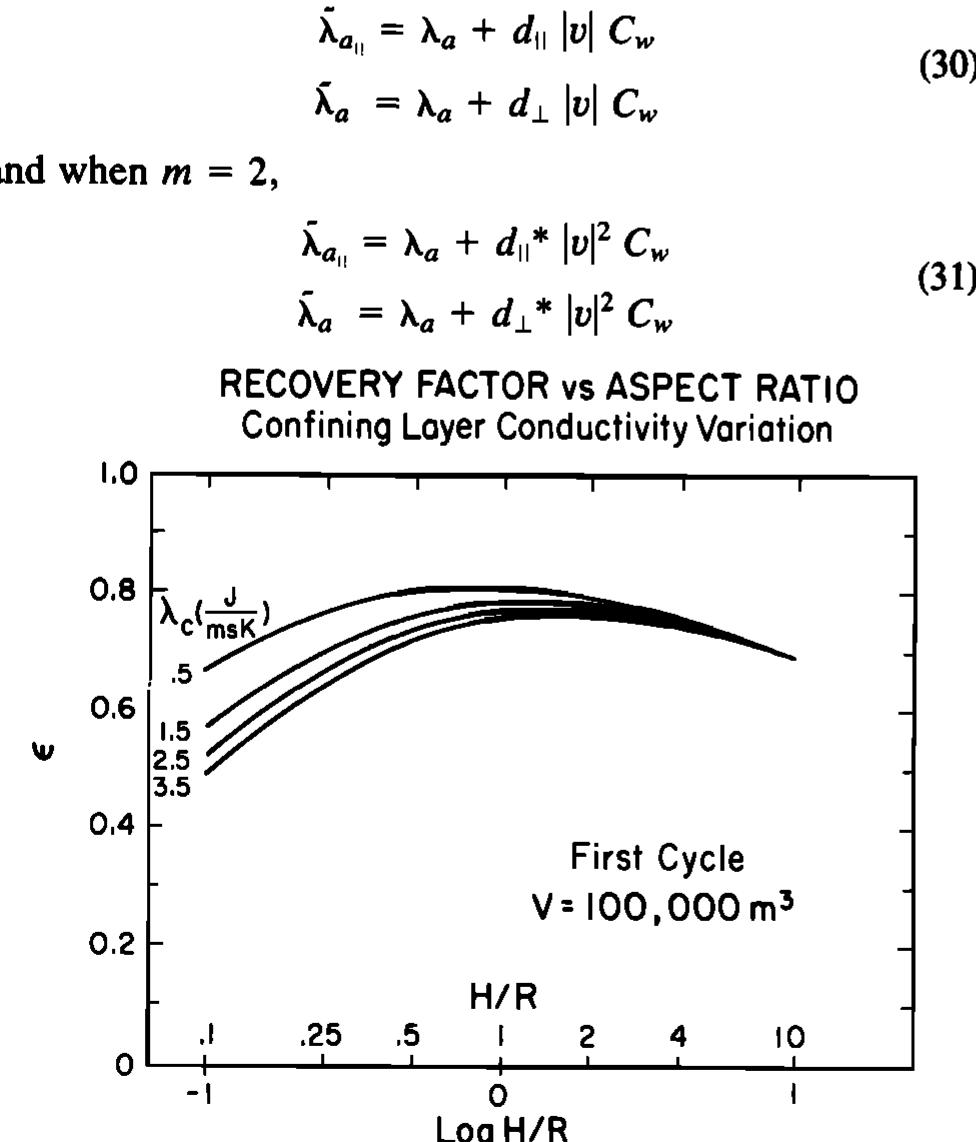
![Fig. 8. Recovery factor for different thermal volumes for the first five cycles and first cycle production temperature versus time for different thermal volumes. 3.2.1. Velocity-dependent dispersion. During periods when the water flows through the aquifer there is, in addition to ordinary heat conduction, a dispersion of heat due to the velocity distribution across each flow channel, the irregular- ity of the pore system, and large-scale aquifer heterogene- ities. According to the theory for dispersion of a nonadsor- bent tracer in uniform porous media [Scheidegger, 1960], the dispersion is proportional to |v,|”, where v, is the pore velocity. The value of m ranges from 1 to 2. When m is 1, the molecular transverse diffusion between adjacent streamlines can be neglected, and when m is 2, the transverse diffusion is important. The transverse diffusion becomes more important as pore velocity decreases. The thermal conductivity of the stagnant liquid-solid mixture and the heat dispersion may be combined to form an effective thermal conductivity. Gener-](https://figures.academia-assets.com/46885808/figure_010.jpg)


![Following the derivation described in “Appendix,” the resistance factor for pile setup (@setup) based on the FOSM Method can be expressed as: where Aseiup is the resistance bias factor of the setup resistance, COVprrop is the coefficient of variation of the resistance at EOD, and COVpgetup is the coefficient of variation of the setup resistance. This equation reveals that Psetup 18 dependent on several parameters. Considering only the AASHTO [3] “Strength I” load combination, the probabilistic characteristics (y, 2, and COV) of the random variables Qp and Q, are defined in Eq. (4). Considering the database of steel H-piles summarized in Table 1, the probabilistic characteristics (4 and COV) of the random variables Reop and Ryeup were selected from RR4 and RR; of Table 2, respectively. Since the « value is suggested as unity in the “Appendix,” the following analyses primarily focus on the influence of the remaining parameters (i.e., 7, (EOD; and QOp/Qz) on setup:](https://figures.academia-assets.com/44065741/figure_003.jpg)


![Fig. 7 Comparison of @etup based on FOSM and FORM for (a) £7 = 2.33, and (b) Br = 3.00 while the pile performance in terms of achieving the desired Riarget 18 verified using either a dynamic analysis method such as WEAP or SLT. The target nominal pile resistance estimated using a static analysis method (Riargetstatic) 18 determined by: Using the proposed FOSM procedure, Ta rizes the recommended resistance factors for ble 3 summa- both the Skov and Denver’s [24] method and the setup Eq. (3). Com- paring these resistance factors calculated Denver’s [24] method and all pile types (..e., for Ro; 0.27 and 0.20 for Rsetup), higher resi were obtained for the setup Eq. (3) and stee higher resistance factors are attributed to (1) t for Skov and 0.58 and 0.45 stance factors H-piles. The he application of a more accurate empirical pile setup Eq . (3) as dem- onstrated in Ng et al. [19], and (2) the use of the regional database given in Table 1, which contained only steel H-piles, hence reducing the uncertainties caused by various pile types used by Yang and Liang [27]. However, it is important to remind that Eq. (3) was developed based on load tests performed within 36 days, the recommended resistance factors shall be used with caution for a pile setup estimated longer than 36 days. Furthermore, the recom- mended (gop for Eq. (3), 0.78 and 0.65 for fh; of 2.33 and 3.00, respectively, shall be used with caution as they were determined based on a limited sample size pile load test data are available in future, recalibration of the resistance factors using the proposed encouraged. of 8. If more procedure is](https://figures.academia-assets.com/44065741/figure_008.jpg)
![Normalizing the above expression with respect to the total load (Qp + Q,), and further rearrangement of Eq. (21) in terms of the dead load to live load ratio (1.e., Op/ Q,) and representing « as the ratio of pile resistance at EOD to the total load (i.e., « = Reop/[QOp + Qr]), the resistance factor of pile setup at a target reliability index (B7) can be expressed as: The parameter «, a ratio of pile resistance at EOD to total load, noted above is analogous to a safety factor applied to the Reop if the traditional allowable stress design (ASD) approach would have been considered. The uncertainties associated with Rgop have been accounted for in terms of @gop in Eq. (22) to comply with the LRFD approach. Since the uncertainties were addressed, the parameter « is suggested as unity in order to eliminate the redundancy in the safety margin applied to Rgop, and the resistance factor for pile setup based on the FOSM method can be expressed as:](https://figures.academia-assets.com/44065741/figure_009.jpg)


![* Based on a suggested « value of one; ° based on Yang and Liang’s [27] results; and © based on a sample size of 8 and use with caution Table 3 Summary of recommended LRFD resistance factors](https://figures.academia-assets.com/44065741/table_003.jpg)
![Table 4 Summary of AASHTO [3] recommended LRFD resistanc« factors static analysis methods (i.e., «method, /-method, A-method, and CPT-method) listed in Table 4. Having a arger denominator term and the same XQ, the Riarget,zoD determined using Eq. (10) considering pile setup will certainly be smaller than the Riargetstatic determined using Eq. (8). If the pile setup is considered and incorporated in design using the proposed LRFD procedure: (1) the target pile driving resistance determined using Eq. (10) will be smaller than that determined using the conventional static analysis method; (2) a shorter pile embedment length will be required to achieve the target pile resistance; (3) the retapping of piles after EOD, for which the assumed target pile driving resistance at EOD based on a static analysis method has not been met, can be reduced since a smaller target pile driving resistance will be required; and (4) the economic advantages of pile setup can be realized while complying with the LRFD framework and ensuring a target reliability level. The aforementioned advantages have been confirmed in a recent study that investigated the impact of incorporating setup on 604 production steel H-piles driven in cohesive soils [17]. This study found that the target driving resistance on average was reduced by 17 % and the number of production piles requiring retapping reduced from 37 % to 15 %.](https://figures.academia-assets.com/44065741/table_004.jpg)


![Figure £. tM -4, System Architecture |O}. It is important that prior of using HDM-4 for the first time in any country, the system should be configured and calibrated for local use. In the HDM-4, thus no attempt for calibration without calibration, however, HDM-4 relationships predict “average expected” values for various variables that can naturally involve large margins of error depending on the situation. Thus the study will produce only an indicative evaluation of the suitability of HDM-4 as a design tool [7]. The HDM-4 relationships for predicting the time to initiation and progression of all structural cracking are as follows: Among the most answered models for optimization of road maintenance is HDM4. It is a powerful system: When considering the applications of HDM-4, it is necessary to look at the highway management process in terms of the following functions [6]: (Planning; Programming; Preparation and Operations). 3- Highway development and management model (HDM-4)](https://figures.academia-assets.com/40151603/figure_001.jpg)


![Fig. 2. Comparison of measured periods with those calculated using eq. [2] for steel moment resisting frame buildings. Fig. 2 for 53 steel frame buildings in two orthogonal direc- tions, providing measured data for 103 cases. — computed as 1.7, 3.7, and 5.7 s, respectively. The same buildings were computed to have fundamental periods of 0.7, 1.2, and 1.6 s, respectively, based on eq. [1] (the 2005 NBCC equation). The analytically computed values were 2.4-3.6 times the values computed by the expression given in the 2005 NBCC, indicating that analytically computed pe- riods could be significantly longer. The results also indicate that the computed values approach those empirically deter- mined by eq. [1] when the bracing effects of nonstructural infill walls are considered. It was found that a few nonstructural masonry infill walls were sufficient to signifi- cantly shorten the fundamental period of low- to medium- rise frame buildings to approximately the levels given by eq. [1] when the walls were not well separated from the lat- eral force resisting system. Therefore, designers should exer- cise caution when using bare frame models for the computation of fundamental period and ensure that the structure is not braced by nonstructural components that were not considered in structural design, after it is built.](https://figures.academia-assets.com/49241061/figure_001.jpg)
![Fig. 1. Comparison of measured periods with those calculated using eq. [1] for reinforced concrete moment resisting frame buildings](https://figures.academia-assets.com/49241061/figure_002.jpg)
![Fig. 3. Effects of nonstructural masonry infills on fundamental periods of 5-, 10-, and 15-storey reinforced concrete frame buildings when not properly isolated from the frames. Fig. 4. Comparison of measured periods with those calculated using eq. [4] for reinforced concrete shear wall buildings](https://figures.academia-assets.com/49241061/figure_003.jpg)
![when D is substituted in place of D,. Hence, it may be argued that the implied accuracy of eq. [4] may not be justi- fiable. Instead, an expression similar to those recommended for frame buildings may be used for shear wall and braced frame buildings as a function of building height only (Goel and Chopra 1997; Morales and Saatcioglu 2002). Figure 5 shows the correlation of measured periods with the follow- ing equation, which has been adopted by UBC (1997), IBC (2000), and the 2005 NBCC: walls in the structure. The 1995 NBCC specifies the funda- mental period of such structures as a function of the length of braced frames or shear walls and building height as fol- lows:](https://figures.academia-assets.com/49241061/figure_004.jpg)

![Fig. 5. Comparison of measured periods with those calculated using eq. [5] for reinforced concrete shear wall buildings seismicity with I,F,5,(0.2) =0.35; and (iii) all buildings that have rigid diaphragms and are torsionally sensitive.](https://figures.academia-assets.com/49241061/figure_006.jpg)


![Figure 4. Flowchart of methods in the ModC lark method In which, S,,) is the reservoir at time t, O, the output of the reservoir at time t, and K is the Clark reserve coefficient. In this study, software based on the ModClark method and developed by Alvankar et al. (2006) in the Visual Basic environment has been used [25]. By examining the available data, seven rainfall events with accessible rainfall-runoff information were selected. For calibration and validation of the incident model, the events were classified into two categories and five events were selected for calibration and two events for validation. At the time of the occurrence of each flood, by using the daily precipitation recorded at the rain gauge stations inside and around the Tangrah watershed, the spatial distribution of the storms was extracted using an Inverse Distance Weighted (IDW) method in the GIS environment. The time distribution of the storms was also determined using the rain gauge data recorded at the Golestan National Park's rain gauge station. The time of concentration of the Tangrah watershed was calculated using the Bransby Williams method (recommended for basins larger than 50 square miles). The reserve coefficient was used by a graphical method [26] and as a preliminary estimation in the calibration step. The watershed curve number was also calibrated using a coefficient. The steps in implementing the Clark model are presented in Figure 4.](https://figures.academia-assets.com/55935535/figure_004.jpg)


![Table 2.6 Anchorage Ratio Criteria [API650, 2007] mechanically anchored.](https://figures.academia-assets.com/37615588/figure_045.jpg)

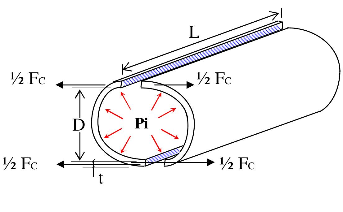
![The maximum longitudinal shell compression stress, 6, is calculated to be 12.69 N/mm?, allowable stress Fc, which can be determined as follow [API 650, 2007]: The calculated maximum longitudinal shell compression stress has to be less than the](https://figures.academia-assets.com/37615588/figure_047.jpg)


![Figure 1.3 Types of Fixed Roof Tanks [EEMUA 2003, vol.1, p.11] Figure 1.3 shows the three types of Fired Roof Tanks.](https://figures.academia-assets.com/37615588/figure_003.jpg)

![Figure 1.5 Double Deck Type Floating Roof [Bob. L & Bob. G, n.d, p.155]](https://figures.academia-assets.com/37615588/figure_005.jpg)

![Figure 1.7 Double Deck Floating Roof Tank [EEMUA 2003, vol.1, p.15]](https://figures.academia-assets.com/37615588/figure_007.jpg)


![Figure 1.11 Tank Exploding [Bob.L & Bob.G, n.d, p.26] 2.11 Tank Shell Design Method as Per API 650](https://figures.academia-assets.com/37615588/figure_012.jpg)

![Figure 1.13 Rotation of the shell-to-bottom connection [Bob.L & Bob.G, n.d, p.47] hydrostatic load.](https://figures.academia-assets.com/37615588/figure_014.jpg)

![Figure 1.15 Floating roof overtopped [Praveen, 2006]](https://figures.academia-assets.com/37615588/figure_016.jpg)
![Figure 1.20 Tank Farm on Fire [Praveen, 2006]](https://figures.academia-assets.com/37615588/figure_017.jpg)

![Figure 1.18 Elephant-foot buckling (broad tanks) [Praveen, 2006] And one case on Tank Farm/ Plant](https://figures.academia-assets.com/37615588/figure_019.jpg)
![Figure 1.19 Tanks Burn Down [John, 2006]](https://figures.academia-assets.com/37615588/figure_020.jpg)


![Figure 1.28 Bleeder vents [EEMUA 2003, vol.1, p.15] [he number and size of the bleeder vent shall be sized accordance to the maximum filling](https://figures.academia-assets.com/37615588/figure_028.jpg)


![Figure 2.12 Design Response Spectral for Ground-Supported Liquid Storage Tanks [API650, 2007] The first mode sloshing wave period (Tc), in second is calculated by the following](https://figures.academia-assets.com/37615588/figure_038.jpg)
![It was defined in API 650 (2007) that for regions outside U.S.A, Ty shall be taken as 4 seconds [API650, 2007].](https://figures.academia-assets.com/37615588/figure_039.jpg)


![Figure 2.16 Center of Action for Effective Forces [API650, 2007] 3.2.8.7 Ring Wall Moment](https://figures.academia-assets.com/37615588/figure_043.jpg)


![Figure 3.3 Minimum Requirement for Single Deck Pontoon Floating Roof [EEMUA 2003, vol.1 p118]](https://figures.academia-assets.com/37615588/figure_052.jpg)


![Figure 3.29 General Arrangement of the Multiple Foam Chamber on the Floating Roof Tank [NFPA 11, P53]](https://figures.academia-assets.com/37615588/figure_084.jpg)

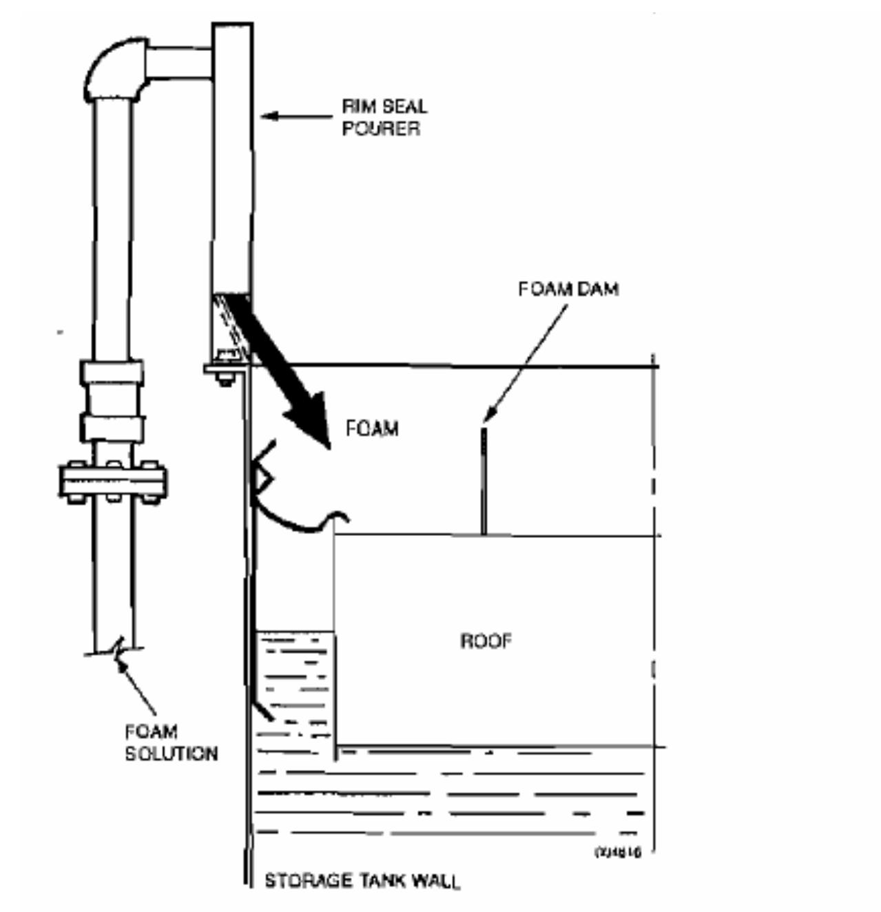
![Figure 3.31 Typical Foam Dam [NFPA 11, p20]](https://figures.academia-assets.com/37615588/figure_086.jpg)


![Figure 4.1 (b) Jacking-Up and Flotation Method for Welded Vertical Tank [PTS, 1986]](https://figures.academia-assets.com/37615588/figure_089.jpg)

![Figure 4.3 Bottom Plate Layout [PTS, 1986]](https://figures.academia-assets.com/37615588/figure_091.jpg)


![Figure 5.2 Maximum Tolerances for Out-of Verticality of the Tank Shell [EEMUA 2003, vol.1, p81] significant influence to the roof rim and rim seals design.](https://figures.academia-assets.com/37615588/figure_099.jpg)


![Table 1.6 Material Selection Guide [Moss, cited in Bednar 1991] available and cost effective material.](https://figures.academia-assets.com/37615588/table_003.jpg)

![Table 1.8 (b) Fitting Requirement on Floating Roof [PTS, 1986] Table 1.8 (a) Fitting Requirements on Tank Shell [PTS, 1986]](https://figures.academia-assets.com/37615588/table_005.jpg)


![Mapped Maximum Considered Earthquake Spectral Response Acceleration at 1 Sec Periods Table 2.3 Value of Fv as a Function of Site Class [AP1I650, 2007] For site class of D and S; as 1.25 Sp, where Sp = 0.3g, S; = 0.375, Fa is to be](https://figures.academia-assets.com/37615588/table_010.jpg)

![Table 3.4 Properties of Common Seal Material [EEMUA 2003, vol.1, p118]](https://figures.academia-assets.com/37615588/table_012.jpg)


![Fig. 1. Rate of alite hydration as a function of time given by isothermal calorimetry measurements. Chemical analyses of the solution phases [35-39] have furnished persuasive evidence that C3S dissolves congruently and quite rapidly in the first seconds after wetting. In dilute suspensions of C3S, for example, the increase in silicate concentration over the first 30s suggests that the dissolution rate may be at least 10 umol m~?s~! [27]. Stein [40] calculated a theoretical solubility product for C3S of K,) 3, when referenced to Eq. (1), which would imply that C3S should continue to dissolve until reaching equilibrium calcium and silicate concentrations in solution of several hundred mmol/L. In fact, it is well known that C3S dissolution rates decelerate very quickly while the solution is still undersaturated, by about 17 orders of magnitude with respect to the ion activity product of Reaction (1)](https://figures.academia-assets.com/67367308/figure_001.jpg)
![Fig. 2. Concentrations of silica (y-axis in mol/L) and calcium (x-axis in mmol/L) reported for cement paste pore solution, collected from an extensive literature search in [44], and interpreted as indicating that either of two types of C-S-H can establish equilibrium with the solution.](https://figures.academia-assets.com/67367308/figure_002.jpg)
![Fig. 3. Progression of hydrogen concentrations with depth and time during the initia! and slow reaction periods for triclinic C3S hydrated at 30 °C [49].](https://figures.academia-assets.com/67367308/figure_003.jpg)

![Fig. 5. Cross-section of a solubility diagram in the system CaO-SiO,-H,0. The arrow shows the path followed by the concentrations in solution during the congruent dissolution of C3S. The concentration increases beyond the solubility of C-S-H until the maximum supersaturation from which C-S-H precipitates immediately is reached (point A). From [35,126]. Evidence supporting this view comes from studies of dissolution rates of C3S in stirred suspensions [58]. Increases in Ca and Si concentrations in solution were monitored continuously in suspen- sions of C3S so dilute (w/s = 50,000) that, theoretically, the solution should never become supersaturated with respect to C-S-H. Without the complicating factor of C-S-H nucleation and growth, congruent dissolution caused the concentrations of Ca and Si to increase continuously in a 3:1 ratio. With this technique, initial C3S dissolution](https://figures.academia-assets.com/67367308/figure_005.jpg)

![Fig. 7. Plots of bound water index (BWI) versus time for C3S hydration measured by quasi-elastic neutron scattering [31].](https://figures.academia-assets.com/67367308/figure_007.jpg)
![Fig. 8. Heat evolution rate curves during the hydration of C3A (L1) in solutions saturated with respect to portlandite (liquid-to-solid mass ratio = 25) carried out with increasing quantities of gypsum, from [105].](https://figures.academia-assets.com/67367308/figure_008.jpg)
![Fig. 9. Grain of C3A in the presence of calium sulfate after 10 min hydration in environmental cell at high accelerating voltage [92].](https://figures.academia-assets.com/67367308/figure_009.jpg)
![Fig. 10. Calorimetry of portland cement with different addition of gypsum. Reprinted, with permission, from theASTM Proceedings (1946), copyright ASTM International, 100 Barr Harbor Drive, West Conshohocken, PA 19428 [108]. These observations indicate the apparent complexity of the interactions between the alite and aluminate phases during hydra- tion. Such complexity highlights the need for simulation tools that can deal with the interactions among phases through the ions in the pore solution and the occupation of space by the hydrated phases.](https://figures.academia-assets.com/67367308/figure_010.jpg)


![Possible causes of the onset of the N+G period, reproduced from [4]. Table 1](https://figures.academia-assets.com/67367308/table_002.jpg)